POSITION CONTROL OF AN ELECTRO-HYDRAULIC

SERVOSYSTEM

A non-linear backstepping approach

Claude Kaddissi, Jean-Pierre Kenné, Maarouf Saad

École de Technologie Supérieure, 1100 Notre-Dame West street, Quebec H3C 1K3, Canada

Keywords: Electro-hydraulic systems modeling, Non-linear control, Backstepping.

Abstract: This paper studies the control of an electro-hydraulic servosystem using a non-linear backstepping based

approach. These systems are known to be highly non-linear due to many factors as leakage, friction and

especially the fluid flow expression through the servo-valve. Another fact, often neglected or avoided, is

that such systems have a non-differentiable mathematical model for bi-directional applications. All these

facets are pointed out in the proposed model of this paper. Therefore, the control of this class of systems

should be based on non-linear strategies. Many experiments showed the failure of classic control with

electro-hydraulic systems, unless operating in the neighborhood of a desired value or reference signal. The

backstepping is used here to overcome all the non-linear effects. The model discontinuity is solved in this

paper, by approximating the non-differentiable function by a sigmoid, so that the backstepping could be

used without restrictions. In fact, simulation results show the effectiveness of the proposed approach in

terms of guaranteed stability and zero tracking error.

1 INTRODUCTION

An electro-hydraulic system is composed of multiple

components: A pump, which feeds the system with

fluid oil from an oil container; An accumulator,

which acts as an auxiliary of energy integrated in the

hydraulic circuit; A relief valve on the other hand to

compensate the increase of pressure if any; A

hydraulic actuator to drive a given load at a desired

position, its displacement direction, speed and

acceleration are determined by a servo-valve. Note

that oil exiting the hydraulic actuator is driven

through the servo-valve back to the tank.

Electro-hydraulic systems became increasingly

current in many kinds of industrial equipments and

processes. Such applications include rolling and

paper mills, aircraft’s and all kinds of automation

including cars industry where linear movements, fast

response, and accurate positioning with heavy loads

are needed. This is principally because of the great

power capacity with good dynamic response and

system solution that they can offer, as compared to

DC and AC motors. However, as a result of the ever-

demanding complexity with these applications,

considering non-linearity and mathematical model

singularity, the traditional constant-gain controllers

have become inadequate. Lim (1997) applied simple

poles placement for a linearized model of an electro-

hydraulic system. Plahuta et al. (1997) tried a

retroaction strategy for variable displacement

hydraulic actuator and this by using two cascaded

control loops for position and speed control. Zeng

and Hu (1999) used a PDF algorithm (Pseudo-

Derivative Feedback) where the integrator part of a

PID controller was placed in the direct path.

Experiments and simulations showed that factors

resulting in dynamic variations are beyond the

capacity of these controllers. And there are also

many of these factors to take into account, such as

load variations, changes of transducers

characteristics and properties of the hydraulic fluid,

changes of servo components dynamics and other

system components, etc. As a result, many robust

and adaptive control methods have been used. Yu

and Kuo (1996) employed an indirect adaptive

controller for speed feedback, based on pole

placement. Sliding mode controller has been used by

Fink and Singh (1998), in order to regulate the

pressure drop due to the load across the actuator. On

the other hand fuzzy logic control has been

270

Kaddissi C., Kenné J. and Saad M. (2004).

POSITION CONTROL OF AN ELECTRO-HYDRAULIC SERVOSYSTEM - A non-linear backstepping approach.

In Proceedings of the First International Conference on Informatics in Control, Automation and Robotics, pages 270-276

DOI: 10.5220/0001134402700276

Copyright

c

 SciTePress

employed by Yongqian et al. (1998), the controller

was based on a decision rules matrix of the error.

Results were very closed to neural network based

controller as in Kandil et al. 1999, where learning

was accomplished through the output error retro-

propagation and thus system knowledge was not

necessary. Simulation results in these advanced

strategies were very successful in most cases, aside

minor transient state problems or small steady state

error. However, stability is not guaranteed in these

approaches. This is because in such cases stability is

studied on discrete domains and one cannot expect

system behaviour at limits. Another point to consider

is that in spite of ensuring system robustness, most

control strategies might generate a control law with

high amplitude, which causes system saturation.

Such is the case of feedback linéarizations.

Therefore one should think to benefit of system non-

linearities that offer more manoeuvrability to avoid

saturating control signals.

This paper proposes a backstepping approach,

tacking into account all system non-linearities. A

major advantage of the backstepping approach is its

flexibility to build a control law by avoiding the

cancellation of useful non-linearities. In addition

modification is brought so the system model can be

used for bi-directional applications. Under such

modification the use of this approach ensures global

stability of the system, and generates low amplitude

control signal.

The paper is organised as follow. Section 2 presents

the dynamic model of the electro-hydraulic system

with emphasis on non-linearity and non-

differentiability. In section 3, we shall present the

design of a backstepping control strategy according

to the system properties. In section 4 Simulation

results and comparisons will be done. Some

conclusions will be carried out in the last section.

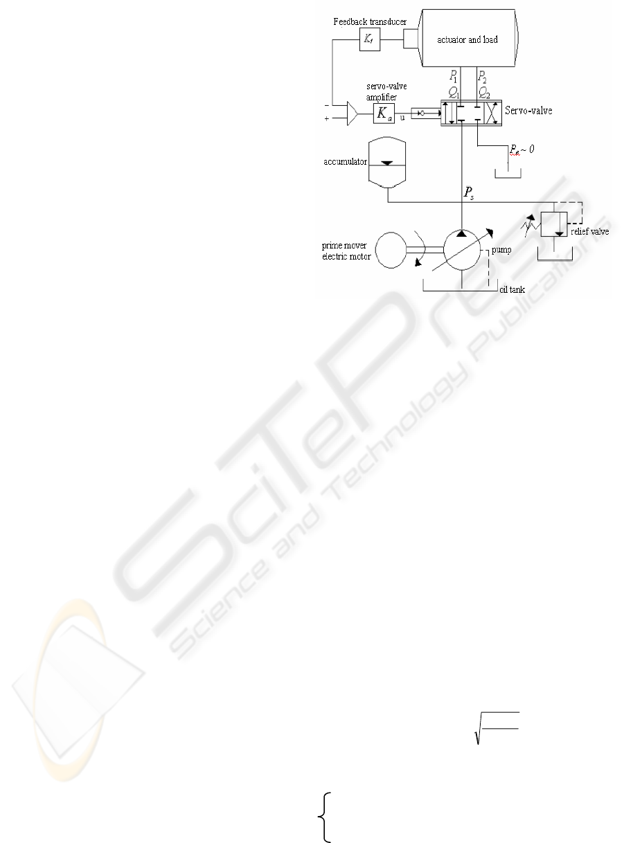
2 SYSTEM MODELING

Consider the hydraulic system shown in figure 1. In

this hydraulic circuit the DC electric motor drives

the pump at constant speed. The pump in turn

delivers oil flow from the tank to the rest of the

components. Normally, the pressure P

s

at the pump

discharge depends on the load, however it is made

constant due to the presence of an accumulator and a

relief valve. In fact, the accumulator acts as an

additional pressure source in case needed. On the

other side the relief valve compensates the pressure

increase due to big loads, by returning the additional

Figure 1: Schematic of hydraulic servo-system

amount of flow to the tank. A hydraulic rotary

actuator drives the load. The actuator rotation is due

to the oil flow coming from the servo-valve, the

latter determines its direction, speed and acceleration

through convenient position of its spool. The control

signal being generated by the controller designed in

this paper actuates the spool to the right position. We

should note that the oil returns to the tank from the

servo-valve at atmospheric pressure and we assume

that the latter is a single stage servo-valve, critically

centred and the orifices are matched and

symmetrical.

The dynamic equation for a servo-valve spool

movement can be given by (LeQuoc et al., 1990):

KuAA

vvv

=+

&

τ

(1)

Where u is the control input, K is the servo–valve

constant,

v

τ

is its time constant and A

v

is the valve

opening area. The flow rate from and to the servo-

valve, through the valve

orifices, assuming small

leakage, are given as:

ρ

Ls

vd

PP

ACQQ

−

==

21

(2)

Where P

L

is the differential pressure due to load.

21

PPP

L

−

=

in the positive direction

12

PPP

L

−

=

in the negative direction

POSITION CONTROL OF AN ELECTRO-HYDRAULIC SERVOSYSTEM - A non-linear backstepping approach

271

21

PPP

s

+=

is the source pressure, C

d

is the flow

discharge coefficient and

ρ

is the fluid oil mass

density.

Since oil viscosity might vary with temperature, it

should be considered in the actuator dynamics along

with oil leakage. Thus we give the compressibility

equation as:

LLm

Lvs

vdL

PCD

PAsignP

ACP

V

−−

−

=

θ

ρβ

&

)(

2

(3)

We define C

L

as the load leakage coefficient,

β

is

the fluid bulk modulus,

θ

is the output angular

position, V is the oil volume under compression in

one chamber of the actuator and D

m

is the actuator

volumetric displacement.

Now we consider the hydraulic actuator equation of

motion given by Newton’s first law. Neglecting the

frictional torque we have:

Lm

TBPPDJ −−−=

θθ

&&&

)(

21

(4)

T

L

is the load torque, B viscous damping coefficient

and J the actuator inertia.

Note that in equations (3) the non-linear term due to

the flow expression and the non-differentiable sign

function that stands for changing in motion direction,

are at the origin of such systems complexity.

Finally choosing,

θ

=

1

x

,

θω

&

==

2

x

,

L

Px

=

3

,

v

Ax =

4

as state

variables; the system can be easily described with a

4th order non-linear state space model.











=

+−=

−−−=

−−=

=

1

44

234343

232

21

)(.

xy

urxrx

xpxpxsignxPxpx

wxwxwx

xx

ba

cbsa

cba

&

(5)

Where r

a

, r

b

, p

a

, p

b

, p

c

, w

a

, w

b

, w

c

, are appropriate

constants given by,

v

a

r

τ

1

=

,

v

b

K

r

τ

= ,

ρ

β

V

C

p

d

a

2

=

,

V

C

p

L

b

β

2

=

,

V

D

p

m

c

β

2

=

,

J

D

w

m

a

= ,

J

B

w

b

= ,

J

T

w

L

c

=

3 BACKSTEPPING BASED

NON-LINEAR CONTROL

In this section, the non-linear backstepping, as

presented by Hassan (2002), will be used to control

the electro-hydraulic system presented in figure 1.

The control law is derived based on a lyapunov

function, to ensure an input-output stability of the

system. This method has been employed before by

Ursu and Popescu (2002) with a reduced order

model of an electro-hydraulic system, for position

control; and with a 4

th

order model for load pressure

control, all with positive desired trajectories or

1)(

4

=

xsign . Later and for better tracking

characteristics the backstepping was applied to a 5

th

order electro-hydraulic system model (Ursu, F. et al.

2003). However the same assumption was held (i.e.

a positive reference for position). Conversely, it is

very vital to consider the case of a trajectory that

takes positive and negative values. Else, the system

application will loose generality, and will bypass a

large number of applications where electro-hydraulic

systems are used. One of those is electro-hydraulic

active suspension, where a hydraulic actuator has to

ensure a minimum vertical displacement of the car

body. Thus, it is evident that under road stochastic

fluctuations, the servo-valve will direct the flow to

the actuator in either ways, depending if the car is

crossing a bump or a pothole. Here, this method will

be used with the system model (5) for position

control and appropriate modification will be brought

to account for a positive-negative varying reference.

We denote by

idii

xxe

−

=

for 4,...,1=i the error

between each state variable and its desired trajectory.

Let us choose a candidate lyapunov function defined

by,

2

11

1

e

V

ρ

=

(6)

Then its derivative is given by,

)()(

1221111111 ddd

xxeexxeV

&&&

&

−+=−=

ρρ

Thus, taking

1112

ekxx

dd

−

=

&

(7)

Renders,

211

2

1111

eeekV

ρρ

+−=

&

(8)

In a second step we shall take,

2

22

12

e

VV

ρ

+=

(9)

ICINCO 2004 - ROBOTICS AND AUTOMATION

272

And its derivative,

22212

eeVV

&

&&

ρ

+=

3222112

2

111

[ ewxweeek

ab

ρρρρ

+−+−=

]

22232 dcda

xwxw

&

ρ

−−+

Here, taking

a

c

a

d

aaa

b

d

w

e

w

k

x

w

e

w

x

w

x +−+−=

2

21

2

1

2

3

1

ρρ

ρ

&

(10)

Will give,

322

2

22

2

1112

eewekekV

a

ρρ

+−−=

&

(11)

Next, consider

2

33

23

e

VV

ρ

+= (12)

Its derivative is given by,

33323

eeVV

&

&&

ρ

+=

2

22

2

111

ekek −−=

ρ

323223

([ xpxpewe

bca

−−++

ρρ

)])()(

34434 ddsa

xxexxsignPp

&

−+−+

By choosing,

34

332

3

2

332

4

)(

xxsignPp

eke

w

xxpxp

x

sa

a

dbc

d

−

−−++

=

ρ

&

(13)

We have,

2

333

2

22

2

1113

ekekekV

ρρ

−−−=

&

34433

)( xxsignPeep

aa

−+

ρ

(14)

Finally we consider,

2

44

34

e

VV

ρ

+= (15)

Next we derive equation (15) and obtain,

44434

eeVV

&

&&

ρ

+=

2

333

2

22

2

111

ekekek

ρρ

−−−=

dba

xurxre

44444

)([

&

ρ

−+−+

])(

3433

xxsignPep

sa

−+

ρ

By setting the control u as stated by equation (16)

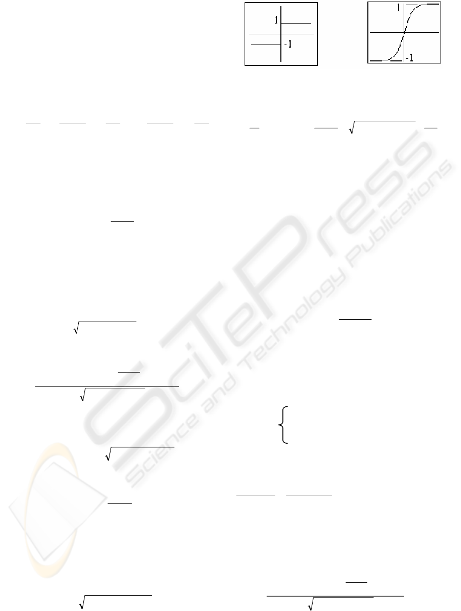
Figure 2: Figure 3:

sign function sigmoid function













−−−+=

4

343

4

3

44

)(

1

e

k

xxsignPe

p

xxr

r

u

s

a

da

b

ρρ

ρ

&

(16)

We should get the following result,

0

2

44

2

333

2

22

2

1114

<−−−−= ekekekekV

ρρ

&

(17)

Unfortunately, this is not the case because the

control signal u is a discontinuous signal, which

involves the derivative of x

4d

that contains a sign(x

4

)

function. Thus it is impossible to generate such

control signal. For that reason and to remedy this

problem, we introduce the sigmoid function defined

by (see figure 2 and 3),

ax

e

xsigm

−

+

−

=

1

)(

(18)

This is a continuously differentiable function with

the following properties,

0>a

1 if

∞→ax

=

)(xsigm 0 if x = 0 (19)

-1 if

−∞→ax

and,

2

)1(

2

)(

ax

e

ae

dx

xdsigm

−

+

=

(20)

Note, that the rate at which sigm(x) converges to 1 or

–1 depends on the slope ‘a/2’.

Now we can rewrite the equation (13) as,

34

332

3

2

332

4

)(

xxsigmPp

eke

w

xxpxp

x

sa

a

dbc

d

−

−−++

=

ρ

&

(21)

Therefore we can solve for control signal u in (16)

by

POSITION CONTROL OF AN ELECTRO-HYDRAULIC SERVOSYSTEM - A non-linear backstepping approach

273

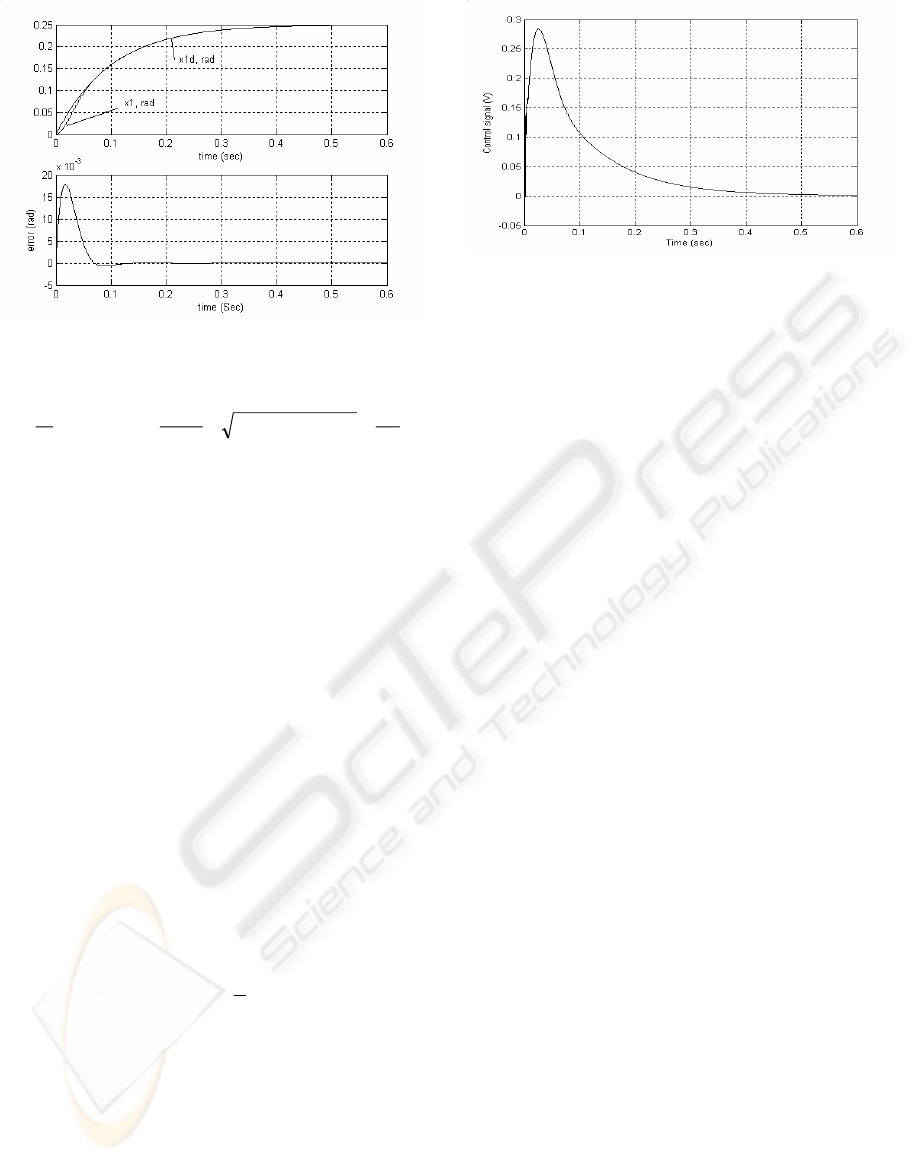
Figure 4: Position vs. desired position and

tracking error













−−−+=

4

343

4

3

44

)(

1

e

k

xxsigmPe

p

xxr

r

u

s

a

da

b

ρρ

ρ

&

(22)

That

gives,

0

2

44

2

333

2

22

2

1114

<−−−−= ekekekekV

ρρ

&

We can state now, that

0

4

<V

&

for every 0

≠

i

e ,

thus we conclude that the control law found in (22)

renders the system globally asymptotically stable.

In the next section we present the simulation of the

controlled system.

4 SIMULATIONS AND RESULTS

We shall present in this section, simulation results to

reveal the backstepping efficiency and robustness in

all cases (see appendix for control parameters

values).

First, let us choose a desired trajectory for position

that tends to a constant,













−=

−

r

t

fd

exx 1

11

> 0 (23)

Thus,

fd

xx

11

→

when ∞→

t

, with a time constant

t

r

. Where we set x

1f

= 0.25rad and t

r

= 0.1 sec.

Graphics are given in figures 4 and 5. Figure 4,

shows how the system output x

1

follows the desired

trajectory with an excellent transient state and a zero

tracking error in steady state. On the other hand

figure 5 shows a smooth control signal generated by

Figure 5: Control signal

equation (22), which drives the servo-valve spool x

4

to the convenient positions, far from saturating

amplitudes. Once desired position reached, x

4

holds

at zero hence no oil will flow to the actuator.

Next we will consider the case of a ‘sine function’

for the desired position with 1 amplitude and 2.5

rad/s frequency. Hence at zero crossing the valve

spool will have to move in the negative direction as

well as the actuator. Figure 6 and 7 shows the

comparison of the control signal when the model in

(5) is simulated with the sign function and the

sigmoid function respectively. It is obvious in the

first case, that when the actuator changes its

direction the discontinuous sign term gives infinite

control amplitude. While, a smooth control is

obtained with the proposed sigmoid function.

Furthermore, as seen from figure 8 the sigmoid

converges exponentially towards a sign with

constant a = 2500.

Finally as seen from figure 9; the

backstepping used with the new system model,

achieves a perfect tracking of the desired position.

This approach is compared with the results of a

classical PID controller based on pole placement. It

is obvious; the PID fails to achieve good tracking,

which results in large steady state error.

We conclude that, the backstepping effectiveness is

not affected by the approximation we made. The

latter allows a smooth continuous control signal as in

figure 7, which justify at the end of our work the

choice for

this approach and the proposition we

brought to the system model.

5 CONCLUSION

In this paper we studied the position control of an

electro-hydraulic servo-system. The control law we

established is based on the non-linear backstepping.

Our goal was to account for the system non-linearity

and non-differentiability, and to show how system

stability is globally guaranteed. We saw how

mathematical model non-differentiability prohibits

ICINCO 2004 - ROBOTICS AND AUTOMATION

274

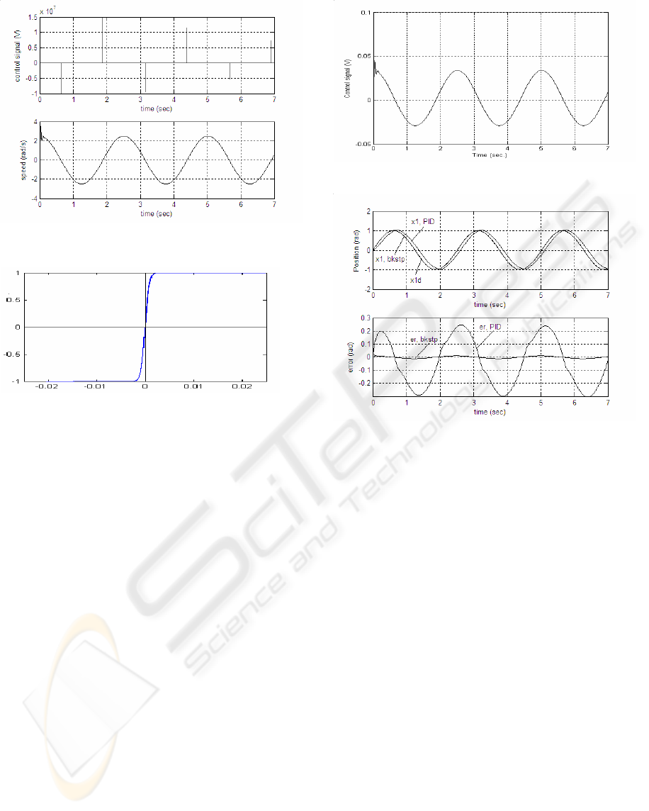
Figure 6: Control signal and actuator speed when

sign function is used

Figure 8: sigm(x

4

) compared to sign(x

4

)

successful control. Introducing the sigmoid function

brought solution to the non-differentiable aspect and

gave the model a smoother expression allowing

successful control via the same strategy. Comparison

with classical PID showed the effectiveness of this

control strategy, as it ensures perfect tracking with

small transient and steady state error. Our future

work consists of real time implementation of this

control law to reveal its effectiveness and bring

improvements if necessary. We are looking as well

to industrial applications of electro-hydraulic

systems, especially in cars industry. Our fields of

interests are basically electro-hydraulic active

suspension control and power transmission control

systems, for better ride quality. Those are the most

competent nowadays applications for hydraulic

servo-systems; especially that road means of

transports are facing a great competition on behalf of

the air and maritime transportations means.

REFERENCES

Fink, A., & Singh, T. (1998). Discrete sliding mode

controller for pressure control with an

electrohydraulic servovalve.

Paper presented at the

control Applications, 1998. Proceedings of the 1998

IEEE International Conference on.

Figure 7: Control signal when sigmoid is used

Figure 9: Position vs. desired position and tracking error

for backstepping and PID

Hassan, K. (2002).

Non-Linear Systems (Third ed.):

Prentice Hall, Upper Saddle River NJ07458.

Kandil, N., LeQuoc, S., & Saad, M. (1999). On-Line

Trained Neural Controllers for Nonlinear Hydraulic

System.

14th World Congress of IFAC, 323-328.

LeQuoc, S., Cheng, R. M. H., & Leung, K. H. (1990).

Tuning an electrohydraulic servovalve to obtain a high

amplitude ratio and a low resonance peak.

Journal of

Fluid Control, 20

(3Mar), 30-49.

Lim, T. J. (1997).

Pole placement control of an

electrohydraulic servo motor.

Paper presented at the

Power Electronics and Drive Systems, 1997.

Proceedings., 1997 International Conference on.

Plahuta, M. J., Franchek, M. A., & Stern, H. (1997).

Robust controller design for a variable displacement

hydraulic motor.

American Society of Mechanical

Engineers, The Fluid Power and Systems Technology

Division (Publication) FPST. Proceedings of the 1997

ASME International Mechanical Engineering

Congress and Exposition, Nov 16-21 1997, 4

, 169-176.

Ursu, I., F. Popescu, & Ursu, F. (2003, May 29-31,).

Control synthesis for electrohydraulic servo

mathematical model.

Paper presented at the

Proceedings of the CAIM 2003, the 11th International

Conference on Applied and Industrial Mathematics,

Oradea, Romania.

POSITION CONTROL OF AN ELECTRO-HYDRAULIC SERVOSYSTEM - A non-linear backstepping approach

275

Ursu, I., & Popescu, F. (2002, October 11-13,).

Backstepping control synthesis for position and force

nonlinear hydraulic servoactuators.

Paper presented at

the Book of Abstracts of the CAIM 2002, 10th

International Conference on Applied and Industrial

Mathematics,. Pitesti, Romania, October 11-13, p. 16.

Yongqian, Z., LeQuoc, S., & Saad, M. (1998).

Nonlinear

fuzzy control on a hydraulic servo system.

Paper

presented at the American Control Conference, 1998.

Proceedings of the 1998.

Yu, W.-S., & Kuo, T.-S. (1996). Robust indirect adaptive

control of the electrohydraulic velocity control

systems.

IEE Proceedings: Control Theory and

Applications, 143

(5), 448-454.

Zeng, W., & Hu, J. (1999). Application of intelligent PDF

control algorithm to an electrohydraulic position servo

system.

IEEE/ASME International Conference on

Advanced Intelligent Mechatronics, AIM Proceedings

of the 1999 IEEE/ASME International Conference on

Advanced Intelligent Mechatronics (AIM '99), Sep 19-

Sep 23 1999

, 233-238.

APPENDIX

Table 1: Hydraulic servo-system parameters

Servo-valve time constant

v

τ

3.18x10

-3

sec

Servo-valve amplifier gain K 0.0397cm

2

/V

Flow discharge coefficient C

d

0.63

Fluid bulk modulus

β

7.995x10

3

daN/cm

2

Actuator chamber volume V 135.4 cm

3

Supply pressure P

S

68.94 daN/cm

2

Fluid mass density

ρ

5

10981

85

x

g/cm

3

Leakage coefficient C

L

0.09047 cm

5

/daN.s

Actuator displacement D

m

2.802 cm

3

/rad

Viscous damping coeff. B 0.766 daN.s.cm

Actuator Inertial load J 0.0481 daN.cm.s

2

Actuator load torque T

L

11.2 daN.cm

Table 2: Control parameters

k

1

10

k

2

2.5

k

3

900

k

4

800

1

ρ

400

2

ρ

0.05

3

ρ

0.003

4

ρ

1700

ICINCO 2004 - ROBOTICS AND AUTOMATION

276