
Lightweight Deep Convolutional Network for Tiny Object Recognition
Thanh-Dat Truong
1
, Vinh-Tiep Nguyen
2
and Minh-Triet Tran
1
1
University of Science, Vietnam National University, HCMC, Vietnam
2
University of Information Technology, Vietnam National University, HCMC, Vietnam
Keywords:
Object Recognition, Lightweight Deep Convolutional Neural Network, Tiny Images, Global Average Pooling.
Abstract:
Object recognition is an important problem in Computer Vision with many applications such as image search,
autonomous car, image understanding, etc. In recent years, Convolutional Neural Network (CNN) based mod-
els have achieved great success on object recognition, especially VGG, ResNet, Wide ResNet, etc. However,
these models involve a large number of parameters that should be trained with large-scale datasets on power-
ful computing systems. Thus, it is not appropriate to train a heavy CNN with small-scale datasets with only
thousands of samples as it is easy to be over-fitted. Furthermore, it is not efficient to use an existing heavy
CNN method to recognize small images, such as in CIFAR-10 or CIFAR-100. In this paper, we propose a
Lightweight Deep Convolutional Neural Network architecture for tiny images codenamed “DCTI” to reduce
significantly a number of parameters for such datasets. Additionally, we use batch-normalization to deal with
the change in distribution each layer. To demonstrate the efficiency of the proposed method, we conduct exper-
iments on two popular datasets: CIFAR-10 and CIFAR-100. The results show that the proposed network not
only significantly reduces the number of parameters but also improves the performance. The number of pa-
rameters in our method is only 21.33% the number of parameters of Wide ResNet but our method achieves up
to 94.34% accuracy on CIFAR-10, comparing to 96.11% of Wide ResNet. Besides, our method also achieves
the accuracy of 73.65% on CIFAR-100.
1 INTRODUCTION
Object recognition is one of the important tasks in
computer vision whose objective is to automatically
classify images into many classes. The result of im-
age classification is an essential precondition of many
tasks such as understanding images, image search en-
gine. Current approaches for image classification are
based on machine learning.
Yann LeCun et. al. proposed Convolutional Neu-
ral Network (LeCun et al., 1989) in the early 1990’s
which demonstrates excellent performance at recog-
nition tasks. Several papers have shown that they
can also deliver outstanding performance on more
challenging visual recognition tasks: Ciresan et. al.
(Ciresan et al., 2012) demonstrate state-of-the-art per-
formance on CIFAR-10 dataset. CNN has recently
enjoyed great success in large-scale image recogni-
tion, e.g CNN architecture is proposed by Krizhevsky
et. al. (Krizhevsky et al., 2017a). In 2015, Karen
Simonyan and Andrew Zisserman propose an archi-
tecture (Simonyan and Zisserman, 2014) which im-
proves the performance of the original architecture of
Krizshevsky.
In reality, objects taken from cameras are often
small or even tiny. Object detection is a method to
determine the object location in an image. Object de-
tection pipeline involves the object recognition mod-
ule. For each object proposal region, we need to rec-
ognize the object in this region. And some regions are
quite small or tiny. In the autonomous car, detecting
and recognizing from far away is really challenging
because objects are taken quite small.
In the recent years, lifelogging rapidly becom-
ing a mainstream research topic. With the rich data
captured over a long period of time, it will require
both advanced methods that can provide an insight
of the activities of an individual and systems capable
of managing this huge amount of data. In the lifelog
scenario there will be present several objects of small
sizes, but the object detection part is equally impor-
tant in this scenario.
The recent common methods deal with tiny ob-
ject recognition is to resize a small image into larger
ones and use common networks having the best per-
formance such as VGG (Simonyan and Zisserman,
2014), Inception (Szegedy et al., 2015), ResNet (He
et al., 2016a), etc. to recognize. But the computa-
Truong, T-D., Nguyen, V-T. and Tran, M-T.
Lightweight Deep Convolutional Network for Tiny Object Recognition.
DOI: 10.5220/0006752006750682
In Proceedings of the 7th International Conference on Pattern Recognition Applications and Methods (ICPRAM 2018), pages 675-682
ISBN: 978-989-758-276-9
Copyright © 2018 by SCITEPRESS – Science and Technology Publications, Lda. All r ights reserved
675

tional cost of their method is really large and cannot
be employed in real time. Although GPU with high
performance can deal with this problem, the price of
GPU is really expensive and not suitable for small de-
vices. Furthermore, resizing a tiny image into a large
image really does not get more information of an im-
age. Additionally, training a large network takes a lot
of time and requires the hardware to be really power-
ful enough.
A good solution for this problem is to keep the size
of the image and to build a network with fewer param-
eters but it still has the ability to recognize with high
accuracy. On this basis, we propose a new method
to employ very deep CNN called Lightweight Deep
Convolutional Network for Tiny Object Recognition
(DCTI). Our proposed network has not only fewer pa-
rameters but also high performance on the tiny im-
age. It has both good accuracy and minimal com-
putational cost. Through experiments, we achieved
some good results which are quite effective for multi-
purposes. This is the motivations for us to continue
to develop our method and build many systems which
make use of object recognition such as understanding
image systems, image search engine systems.
Contributions. In our work, we consider in tiny
images with size 32 × 32. We focus on exploiting
local features with small convolutional filters size.
Therefore, we use convolutional filters size 3 × 3. It
fits with tiny images and helps to extract local fea-
tures. Besides that, it helps reducing parameters and
to push network going deeper.
In traditional approaches, the last layers use fully
connected layers to feed feature maps to feature vec-
tors. However, it increases more parameters and leads
to over-fitting. Our network proposes using global av-
erage pooling (Lin et al., 2013) instead of fully con-
nected layers. The purpose of this work is to help the
network directly project significant feature maps into
the feature vectors. Additionally, global average pool-
ing layers do not employ parameters. So it has fewer
parameters and over-fitting is avoided.
In deep networks, small changes can amplify layer
by layer. It leads to change distribution each layer.
This problem is called Internal Covariate Shift. To
tackle this problem, we use Batch-Normalization pro-
posed by Ioffe et. al. (Ioffe and Szegedy, 2015).
Once again, through experiments, we prove batch-
normalization is potential and efficient. It also helps
faster learning.
Additionally, to prevent over-fitting, we use
dropout. In common, dropout is put after fully con-
nected layers. But in our network, we put it after
convolutional layers. Through experiment, this work
helps improving accuracy and to avoid over-fitting.
We also use data augmentation and whitening
data to improve accuracy. Our method only uses
21.33% number of parameters than the state-of-the-
art method (Zagoruyko and Komodakis, 2016). How-
ever, we achieve the accuracy up to 94.34% and
73.65% on CIFAR-10 and CIFAR-100. With our re-
sult we achieved, it proves that our method not only
gets high accuracy but also reduce parameters signif-
icantly.
The rest of this paper is organized as follows. Sec-
tion 2 presents related works. The proposed architec-
ture of our network is presented in Section 3. Section
4 presents our experimental configuration on CIFAR-
10 and CIFAR-100. We compare our results to other
methods in section 5. Finally, Section 6 concludes the
paper.
2 RELATED WORKS
The earlier method for object recognition named Con-
volutional Neural Networks is proposed by Yann Le-
cun et. al. (LeCun et al., 1989). It demonstrates
high performance on MNIST Dataset. Many current
architectures used for object recognition are based
on Convolutional Neural Networks (Graham, 2014),
(Krizhevsky et al., 2017a), (Zeiler and Fergus, 2013).
Very Deep Convolutional Neural Networks: a
method proposed by Andrew Zisserman et. al. (Si-
monyan and Zisserman, 2014). It has good perfor-
mance on ImageNet Dataset. Very deep convolu-
tional neural networks have two main architectures
are VGG-16 and VGG-19. VGG-16 and VGG-19
mean that there are 16 layers and 19 layers having
parameters. The main contribution of its paper is a
thorough evaluation of networks of increasing depth
using an architecture with very small (3 × 3) convo-
lution filters, which shows that a significant improve-
ment on the prior-art configurations can be achieved
by pushing the depth to 16-19 weight layer.
Network In Network: notice the limitations of
using the fully connected layer, a novel network struc-
ture called Network In Network (NIN) to enhance the
model discriminability for local receptive fields (Lin
et al., 2013). Global average pooling is used in this
network instead of fully connected layer. The pur-
pose of this work is to reduce parameters and enforc-
ing correspondences between feature maps and cate-
gories. It continues improving by Batch-normalized
Maxout and has good performance on CIFAR-10
dataset (Chang and Chen, 2015). In our work, we
also use global average pooling approach.
Deep Residual Learning for Image Recogni-
tion: one of the limitations when the network has
INDEED 2018 - Special Session on INsights DiscovEry from LifElog Data
676
more layers is the gradient is vanished in back-
propagation process. To avoid this problem, a method
proposed by Kaiming He (He et al., 2016a). It
presents a residual learning framework to easy the
training of networks that are substantially deeper than
those used previously. Deep Residual gets high per-
formance on ImageNet dataset, CIFAR dataset.
Going Deeper with Convolutions: one of the
important works when designing a network is that se-
lects kernels for each layer. Should we use a size of
the kernel of convolutional layers is 1 × 1, 3 × 3 or
5 × 5? To solve this problem, the group of Google’s
authors proposed a method codenamed Inception that
achieves the new state-of-the-art for classification and
detection in the ImageNet Large-Scale Visual Recog-
nition Challenge 2014 (Szegedy et al., 2015). The
idea of the method is to use all three size kernels
each convolutional layer. By a carefully crafted de-
sign, they increase the depth and width of the network
while keeping the computational budget constant.
Deep Networks with Internal Selective Atten-
tion through Feedback Connections: traditional
CNN are stationary and feed-forward. They neither
change their parameters during evaluation nor use
feedback from higher to lower layers. Real brains,
however, do. So does the Deep Attention Selective
Network (DasNet) architecture. DasNet’s feedback
structure can dynamically alter its convolutional fil-
ter sensitivities during classification. It harnesses the
power of sequential processing to improve classifica-
tion performance, by allowing the network to itera-
tively focus its internal attention on some of its con-
volutional filters (Stollenga et al., 2014).
Recurrent Convolutional Neural Network for
Object Recognition: a prominent difference is that
CNN is typically a feed-forward architecture while
in the visual system recurrent connections are abun-
dant. Inspired by this fact, its paper proposes a recur-
rent CNN (RCNN) for object recognition by incorpo-
rating recurrent connections into each convolutional
layer (Liang and Hu, 2015).
3 PROPOSED ARCHITECTURE
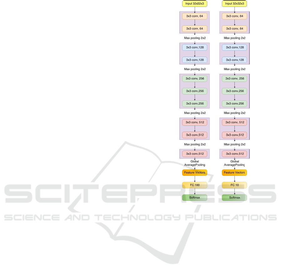
3.1 Overall Architecture
DCTI has 5 phases of convolutional layers (see Fig-
ure 1). We use all filters with receptive field 3x3
for all convolutional layers. All hidden layers are
equipped with the rectification (ReLUs (Krizhevsky
et al., 2017b)) non-linearity. We use dropout and
batch-normalization after each convolutional layer.
Figure 1: Overall architecture of Lightweight Deep Con-
volutional Network for Tiny Object Recognition (top for
CIFAR-10, bottom for CIFAR-100).
From the original image size 32 × 32 and 3 color
channels, we process multiple phases, after each
phase, we use max pooling with the pool size 2 × 2
to reduce the size of feature maps down to two times.
The purposes of this work are to reduce variance, re-
duce computation complexity (as 2 × 2 max pooling
reduces 75% data) and extract low level features from
a neighborhood. Through four max pooling layers,
we receive feature maps with the size 2 × 2.
In the first phase, the current input size is 32 ×32.
Therefore, we use convolutional filters size 5 × 5 to
deal with detail local features. Instead of using one
convolutional layer with the kernel size 5 × 5, we use
two convolutional layers with kernel size 3×3. Using
two convolutional filers size 3 × 3 is equivalent to one
convolutional filter size 5 × 5. By this way, we reduce
parameters and push network going deeper.
In the second phase, the current input size is
16 × 16. We continue processing local feature with
convolutional filter size 5 × 5 on all feature maps. We
implement this by 2 convolutional layers with kernel
size 3 × 3. The similarity with the first phase, using
2 convolutional filters help reducing parameters and
Lightweight Deep Convolutional Network for Tiny Object Recognition
677

increase more layers.
In the third phase, the current input size is 8 × 8.
We want to hold on global feature maps, so we use
convolutional filters 7 × 7. We implement by three
convolutional layers with the kernel size 3 × 3, it is
equivalent to one layer 7 × 7. We incorporate three
non-linear rectification layers instead of a single one,
which makes the decision function more discrimina-
tive. Second, we decrease the number of parame-
ters than use one convolutional layers with kernel size
7 × 7. This can be seen as imposing a regulariza-
tion on the 7 × 7 convolutional filters, forcing them
to have a decomposition through the 3x3 filters (with
non-linearity injected in between).
In the fourth and fifth phases, the input sizes are
just 4 × 4 and 2 × 2. We continue dealing with global
features. We use convolutional filters size 5×5 for the
fourth phase and convolutional filters size 3×3 for the
fifth size. It guarantees that convolutional filters still
fit with feature maps. We use two convolutional filters
size 3 ×3 instead of using one convolutional filter size
5×5. Finally, we receive feature maps with size 2×2,
it uses to directly feed to feature vectors.
In final, we use global average pooling layer to
feed directly feature maps into feature vectors. From
feature vectors, we apply fully connected and softmax
to calculate probability each class.
3.2 Data Normalization
Since the range of values of raw data varies widely,
in some machine learning algorithms, objective func-
tions will not work properly without normalization.
Another reason why data normalization is applied is
that gradient descent converges much faster with data
normalization than without it.
Data normalization makes the values of each fea-
ture in the data have zero-mean (when subtracting
the mean in the numerator) and unit-variance. This
method is widely used for normalization in many
machine learning algorithms (e.g., support vector
machines, logistic regression, and neural networks)
(Grus and Joel, 2015). This is typically done by cal-
culating standard scores. (Mohamad et al., 2013) The
general method of calculation is to determine the dis-
tribution mean and standard deviation for each fea-
ture. Next, we subtract the mean from each fea-
ture. Then we divide the values (mean is already sub-
tracted) of each feature by its standard deviation.
3.3 Whitening Transformation
A whitening transformation or sphering transforma-
tion is a linear transformation that transforms a vector
of random variables with a known covariance matrix
into a set of new variables whose covariance is the
identity matrix meaning that they are uncorrelated and
all have variance(Kessy et al., 2015).
We use ZCA whitening transformation
(Krizhevsky, ) to transform our data. We store
d × n − dimensional data points in the columns of a
d × n matrix X. Assuming the data points have zero
mean.
First, we need to compute Σ =
1
n
XX
T
. Next, we
computes the eigenvectors Σ. Suppose matrix U con-
tains the eigenvectors of Σ (one eigenvector per col-
umn, sorted in order from top to bottom eigenvector),
and the diagonal entries of the matrix S will contain
the corresponding eigenvalues (also sorted in decreas-
ing order).
X
ZCAW hite
= U.diag(S)
−
1
2
.U
T
.X
where: diag(S) means diagonal of matrix S. Exponent
−
1
2
means each element of matrix has exponent −
1
2
.
3.4 Rectifier
The most important feature of AlexNet is ReLUs
(Krizhevsky et al., 2017b) nonlinearity, which shows
the importance of nonlinearity. Two additional major
benefits of ReLUs are sparsity and a reduced likeli-
hood of vanishing gradient. But first recall the defini-
tion of a ReLUs is h = max(0, a).
One major benefit is the reduced likelihood of the
gradient to vanish. This arises when a > 0. In this
regime, the gradient has a constant value. In contrast,
the gradient of sigmoids becomes increasingly small
as the absolute value of x increases. The constant gra-
dient of ReLUs results in faster learning.
The other benefit of ReLUs is sparsity. Sparsity
arises when a ≤ 0. The more such units that exist in
a layer the more sparse the resulting representation.
Sigmoids, on the other hand, are always likely to gen-
erate some non-zero value resulting in dense repre-
sentations. Sparse representations seem to be more
beneficial than dense representations.
3.5 Batch Normalization
Batch normalization potentially helps in two ways:
faster learning and higher overall accuracy. The im-
proved method also allows you to use a higher learn-
ing rate, potentially providing another boost in speed.
For very deep networks, small changes in the pre-
vious layers will amplify layer by layer and finally
cause some problem. The change in the distribu-
tion of layer inputs causes problems since the pa-
rameter should adapt to new distribution with itera-
tions, which is called Internal Covariate Shift (Ioffe
INDEED 2018 - Special Session on INsights DiscovEry from LifElog Data
678

and Szegedy, 2015). To solve this problem, Google’s
researcher Ioffe proposed Batch Normalization (Ioffe
and Szegedy, 2015), which normalizes every layer’s
inputs, thus it makes the network converge much
faster, converge at lower error rate and reduce over-
fitting to some degree.
Y = γ
X −µ
σ
+ β
Where: µ = X, σ
2
= (X − µ)
2
, γ, β are learnable pa-
rameters. In our experiment, we set γ = 1 and β = 0.
3.6 Global Average Pooling
This method is proposed by Min Lin et. al. (Lin
et al., 2013). They propose another strategy called
global average pooling to replace the traditional fully
connected layers in CNN. The idea is to generate one
feature map for each corresponding category of the
classification task in the last block of the convolu-
tional layer. Instead of adding fully connected lay-
ers on top of the feature maps, they take the aver-
age of each feature maps, and the resulting vector is
fed directly into the softmax layer. One advantage of
global average pooling over the fully connected lay-
ers is that it is more native to the convolution structure
by enforcing correspondences between feature maps
and categories. Thus the feature maps can be easily
interpreted as categories confidence maps. Another
advantage is that there is no parameter to optimize in
the global average pooling thus over-fitting is avoided
at this layer.
In our architecture, instead of being fed directly
into the softmax layer, we use global average pooling
to extract feature vectors 512-dimension. Global av-
erage pooling sums out the spatial information, thus it
is more robust to spatial translations of the input.
3.7 Dropout
When we use a very deep CNN for small datasets, it
easily tends to over-fitting. The most common meth-
ods reducing over-fitting is dropout (Srivastava et al.,
2014). The standard way of using dropout is to set
dropout at the fully connected layers where most pa-
rameters are. However, the model is very deep and the
dataset is relatively small, we use a different way of
dropout setting. We set dropout for convolution lay-
ers, too. Specifically, we set dropout rate as 0.3 for
the first and second group of convolution layers, 0.4
for the third and fourth group. The dropout rate for
the feature vectors 512D layer was set to be 0.5.
4 EXPERIMENTS
We experiment our method on CIFAR-10 dataset.
Each image we have a vector result with 10-
dimension, each element represents for the proba-
bility of corresponding class. To rate our architec-
ture, we use Cross-Entropy Cost Function as objec-
tive function.
L = −
1
N
N
∑
j=1
10
∑
i=1
t
j
i
ln(y
j
i
) + (1 −t
j
i
)ln(1 − y
j
i
) +
λ
2
∑
||W ||
2
Where t
j
is the target of input j
th
, x
j
is the output j
th
,
W is the parameters, λ is a regularization parameter.
We use Stochastic gradient descent (sgd) to opti-
mize parameters. To reduce time training, we train on
GPU instead of CPU. We implement by MatConvNet
of MatConvNet Team. CIFAR-10 dataset has 60000
images with 6000 images each class. We divide the
dataset into 2 sets are training set and test set. Train-
ing set has 50000 images, test set has 10000 images.
Configurations of computer use for this training are
CPU Core i3 4150, RAM 8GB, GPU GTX 1060 6GB.
The training process takes about 10 hours to train.
We conduct the training model for 500 epochs.
Use mini-batch sgd to solve the net, with batch-size
of 64. The momentum, base learning rate and base
weight decay rate are set to 0.9, 0.1, 0.0005, respec-
tively. Lower down the learning rate every an epoch
by a factor of 0.9817.
To accelerate training process and prevent over-
fitting, we use data augmentation while training. We
flip image left to right with probability is 0.5 and ran-
dom crop with padding is 4 (pads array with mirror
reflections of itself). We also experiment on CIFAR-
100 dataset. We use same experimental configura-
tions with the experiment on CIFAR-10.
In figure 2 , the red line represents for training
and the green line represents for testing. In 250 first
epochs, the objective and accuracy converge quickly
to stabilized result. After the result does not change
too much and the result is stabilized. Through that,
our method can quickly converge to stabilized result
quickly with regular configurations of computer and
takes less time to training (500 epochs take 10 hours
to train). It is equivalent when we train our method on
CIFAR-100 (Figure 3).
5 RESULT
The accuracy we achieve on CIFAR-10 test set is
94.34%. See some true predictions in Figure 4. The
input images are tiny, but our method can classify cor-
rectly. In some case, some classes are similarity such
as dog and cat, automobile and truck, etc. It lead to
Lightweight Deep Convolutional Network for Tiny Object Recognition
679
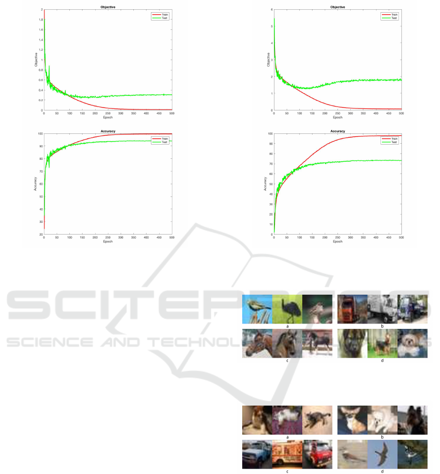
Figure 2: Objective (top) and Accuracy (bottom) training
plot (CIFAR-10).
our method can wrongly classify (see some wrongly
predicted images in Figure 5). Considering in con-
fusion matrix (Table 1), dogs are easily wrongly pre-
dicted as cats, trucks are also easy wrongly predicted
as automobiles or deers are also wrongly predicted as
cats. Because of an abstracted level features, there is
not much difference between these classes.
We compare our architecture to the VGG archi-
tecture. We use fewer parameters than VGG architec-
ture. The number of parameters of our architecture
is about 7.6 million. In while, VGG-16 and VGG-
19 have more than 100 million parameters. Our re-
sult is event better than modified VGG-16 applied to
CIFAR-10 dataset (Liu and Deng, 2015).
We also compare the accuracy of our method with
other methods on CIFAR-10. See the result in Table 2.
Our result uses only 21.33% number of parameters of
the state-of-the-art method but we achieve accuracy
up to 94.34%. Comparing with the other methods
such as VGG, NiN, Dasnet, our method outperform
than their methods. Using only about 7.6M parame-
ters, we reducing parameters significantly and achieve
convincing results.
We also compare our method with the other meth-
ods on CIFAR-100. See the result in Table 3.
Our method performs better than DasNet and NiN
method. Our results are nearly as close to ResNet
1001 method but we use fewer parameters than its
Figure 3: Objective (top) and Accuracy (bottom) training
plot (CIFAR-100).
Figure 4: a) Correctly predicted examples (a) bird (b) truck
(c) horse d) dog.
Figure 5: Same examples of wrongly predicted images (a)
Cats are wrongly predicted as dogs, (b)dogs are wrongly
predicted as cats; (c) trucks are wrongly predicted as auto-
mobiles; (d) birds are wrongly predicted as airplanes.
method. Although our result does not reach the state-
of-the-art, by our method we reduce parameters sig-
nificantly. Specifically, out method has fewer param-
eters than the state-of-the-art method 4.5 times. Ad-
ditionally, we also reach good accuracy and low com-
putational cost.
To achieve this result, we use very small convolu-
INDEED 2018 - Special Session on INsights DiscovEry from LifElog Data
680
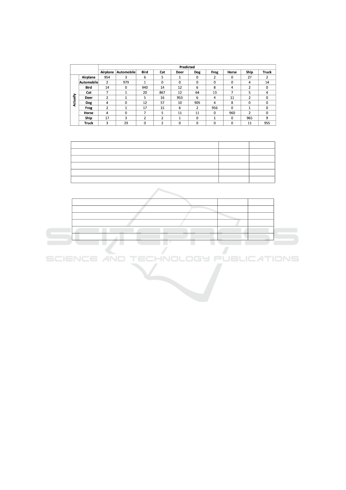
Table 1: Confusion matrix (CIFAR-10).
Table 2: Some results of the comparative experiments (CIFAR-10).
Method Accuracy Params
Wide Residual Networks (Zagoruyko and Komodakis, 2016) 96.11% 36.5M
DCTI 94.34% 7.63M
CIFAR-VGG-BN-DROPOUT (Liu and Deng, 2015) 91.55% 14.7M
NiN (Lin et al., 2013) 91.20% 1.00M
DasNet (Stollenga et al., 2014) 90.78% 1.00M
Table 3: Some results of the comparative experiments (CIFAR-100).
Method Accuracy Params
Wide Residual Network (Zagoruyko and Komodakis, 2016) 81.15% 36.5M
ResNet 1001 (He et al., 2016b) 77.29% 10.2M
DCTI 73.65% 7.68M
DasNet (Stollenga et al., 2014) 66.22% 1.00M
NiN (Lin et al., 2013) 64.32% 1.00M
tional filters size to deal with local features and push
network can going deeper. And the network can learn
high level features. Furthermore, we use global av-
erage pooling helps reducing parameters significantly
and is more native to the convolution structure by en-
forcing correspondences between feature maps and
feature vectors. The new way of putting dropout after
convolutional layers help improving accuracy. It was
proved through our result we achieved.
6 CONCLUSION
In our research, we proposed a new method for object
recognition with tiny images. By using very small
convolutional filters, we pushed our network going
deeper and dealt with local features. It also helped
our network learn high level features. And by using
global average pooling instead of fully connected lay-
ers, we reduced parameters significantly. Moreover,
it helped the network directly project significant fea-
ture maps into the feature vectors. Beside that, us-
ing batch-normalization and dropout helped to accel-
erate the learning process and preventing over-fitting.
Furthermore, it also improved performance and re-
duced computational cost. Although we cannot reach
the state-of-the-art, the results we achieved proved
that our method is promising. It was also demon-
strated that the representation depth is beneficial for
the recognition. Additionally, we proved very deep
models were used to fit small datasets as long as the
input image is big enough so that it does not van-
ish as the model going deeper. Our results yet again
confirmed the performance of very deep CNN for the
pattern recognition task. In the future, we continue
improving our method to get higher performance and
reduce parameters.
REFERENCES
Chang, J. and Chen, Y. (2015). Batch-normalized maxout
network in network. CoRR, abs/1511.02583.
Ciresan, D. C., Meier, U., and Schmidhuber, J. (2012).
Multi-column deep neural networks for image classi-
fication. In CVPR, pages 3642–3649. IEEE Computer
Society.
Graham, B. (2014). Fractional max-pooling. CoRR,
abs/1412.6071.
Grus and Joel (2015). Data science from scratch. CA:
O’Reilly. pp. 99, 100. ISBN 978-1-491-90142-7.
Lightweight Deep Convolutional Network for Tiny Object Recognition
681

He, K., Zhang, X., Ren, S., and Sun, J. (2016a). Deep resid-
ual learning for image recognition. In CVPR, pages
770–778. IEEE Computer Society.
He, K., Zhang, X., Ren, S., and Sun, J. (2016b). Identity
mappings in deep residual networks. In ECCV (4),
volume 9908 of Lecture Notes in Computer Science,
pages 630–645. Springer.
Ioffe, S. and Szegedy, C. (2015). Batch normalization: Ac-
celerating deep network training by reducing internal
covariate shift. In ICML, volume 37 of JMLR Work-
shop and Conference Proceedings, pages 448–456.
JMLR.org.
Kessy, A., Lewin, A., and Strimmer, K. (2015). Optimal
whitening and decorrelation. arXiv.
Krizhevsky, A. Appendix a of learning multiple layers of
features from tiny images.
Krizhevsky, A., Sutskever, I., and Hinton, G. E. (2017a).
Imagenet classification with deep convolutional neu-
ral networks. Commun. ACM, 60(6):84–90.
Krizhevsky, A., Sutskever, I., and Hinton, G. E. (2017b).
Imagenet classification with deep convolutional neu-
ral networks. Commun. ACM, 60(6):84–90.
LeCun, Y., Boser, B. E., Denker, J. S., Henderson, D.,
Howard, R. E., Hubbard, W. E., and Jackel, L. D.
(1989). Backpropagation applied to handwritten zip
code recognition. Neural Computation, 1(4):541–551.
Liang, M. and Hu, X. (2015). Recurrent convolutional neu-
ral network for object recognition. In CVPR, pages
3367–3375. IEEE Computer Society.
Lin, M., Chen, Q., and Yan, S. (2013). Network in network.
CoRR, abs/1312.4400.
Liu, S. and Deng, W. (2015). Very deep convolutional
neural network based image classification using small
training sample size. In ACPR, pages 730–734. IEEE.
Mohamad, B., Ismail, and Usman, D. (2013). Standardiza-
tion and its effects on k-means clustering algorithm.
Simonyan, K. and Zisserman, A. (2014). Very deep con-
volutional networks for large-scale image recognition.
CoRR, abs/1409.1556.
Srivastava, N., Hinton, G. E., Krizhevsky, A., Sutskever, I.,
and Salakhutdinov, R. (2014). Dropout: a simple way
to prevent neural networks from overfitting. Journal
of Machine Learning Research, 15(1):1929–1958.
Stollenga, M. F., Masci, J., Gomez, F. J., and Schmidhuber,
J. (2014). Deep networks with internal selective at-
tention through feedback connections. In NIPS, pages
3545–3553.
Szegedy, C., Liu, W., Jia, Y., Sermanet, P., Reed, S.,
Anguelov, D., Erhan, D., Vanhoucke, V., and Rabi-
novich, A. (2015). Going deeper with convolutions.
In Computer Vision and Pattern Recognition (CVPR).
Zagoruyko, S. and Komodakis, N. (2016). Wide residual
networks. In BMVC.
Zeiler, M. D. and Fergus, R. (2013). Stochastic pooling for
regularization of deep convolutional neural networks.
CoRR, abs/1301.3557.
INDEED 2018 - Special Session on INsights DiscovEry from LifElog Data
682
