A Deep Learning based Food Recognition System for Lifelog Images

Binh T. Nguyen

, Duc-Tien Dang-Nguyen

, Tien X. Dang

, Thai Phat

and Cathal Gurrin

Department of Computer Science, University of Science, Vietnam

Insight Centre for Data Analytics, Dublin City University, Dublin, Ireland

Keywords:

Lifelogging, Food Recognition, CNNs, SIFT, SURF, HOG, Food Detection.

Abstract:

In this paper, we propose a deep learning based system for food recognition from personal life archive im-

ages. The system ﬁrst identiﬁes the eating moments based on multi-modal information, then tries to focus

and enhance the food images available in these moments, and ﬁnally, exploits GoogleNet as the core of the

learning process to recognise the food category of the images. Preliminary results, experimenting on the food

recognition module of the proposed system, show that the proposed system achieves 95.97% classiﬁcation

accuracy on the food images taken from the personal life archive from several lifeloggers, which potentially

can be extended and applied in broader scenarios and for different types of food categories.

1 INTRODUCTION

Lifelogging is the process whereby individuals gather

personal data about different aspects of their nor-

mal life activities for different purposes Gurrin et al.

(2014b), such as capturing photos of important daily

events, logging sleep patterns, recording workouts,

keeping records of food consumption or even mood

changes. This collection of personal data about the

individual’s life is typically called a lifelog or per-

sonal life archive. As digital storage is becoming

cheaper and sensing technology is improving contin-

uously, continuous and passive photo capture devices

are now more popular and affordable. These devices

can help us to maintain digital records about our daily

life much efﬁciently.

In the domain of health care, lifelogging can play

an important role in providing historical information

about the person. It can be seen as a tool that monitors

and tracks the quality of our life; our lifelog records

have the potential to tell us if we are sleeping well or

not based on our sleeping patterns, if we have a proper

diet based on our eating behaviour or how well we are

beneﬁting from our workouts via the analysis of calo-

ries burned and heart rate. In addition to automati-

cally keeping a valuable diary of important moments

and events of our life through the use of photos via

wearable lifelogging cameras and/or traditional cam-

eras, visual lifelogs can contain detailed information

about our daily activities. A wearable camera, such

as a SenseCam, can capture around one million im-

ages per year Dang-Nguyen et al. (2017a), recording a

huge amount of visual information about the wearer’s

life including food consumption details. Such food

photos can be leveraged to track nutritional intake of

the individual on a personal level, which can pro-

vide important insights into the individual’s dietary

habits and can also lead to many interesting applica-

tions such as automatic calculator of food consump-

tion or personalised food recommendation systems.

Monitoring the nutrition habits of a person is an es-

tablished mechanism typically used in the health do-

main for several medical conditions such as obesity,

hypertension and diabetes A. (1992). Utilising the vi-

sual food information available in one’s lifelog can

effectively replace traditional methods of food con-

sumption analysis that currently depend mainly on

subjective questionnaires, manual surveys and inter-

views Liu et al. (2012). This can both make the pro-

cess easier to the user, as well as providing objective

results with fewer errors when compared to conven-

tional manual food monitoring methods.

Considering the food recognition problem, it has

been broadly investigated for many years and there

have been several systems as well as datasets related

to this problem. In FoodAI

, authors study a Singa-

porean food recognition and health care system by

using a deep learning approach. Similarly, CLAR-

IFAI

is constructed for recognizing Western foods.

http://foodai.org

http://blog.clarifai.com

Nguyen, B., Dang-Nguyen, D-T., Dang, T., Phat, T. and Gurrin, C.

A Deep Learning based Food Recognition System for Lifelog Images.

DOI: 10.5220/0006749006570664

In Proceedings of the 7th International Conference on Pattern Recognition Applications and Methods (ICPRAM 2018), pages 657-664

ISBN: 978-989-758-276-9

657

Eating

Moments

Detection

Images

Enhancement

Food

Recognition

Figure 1: The proposed schema of the food recognition system.

Lukas Bossard Lukas et al. (2014) and colleagues pro-

posed a novel approach by using Bag Of Words, Im-

proved Fisher Vector and Random Forests Discrim-

inative Component Mining for building a food de-

tection system. In addition, they also contribute a

large dataset of 101,000 images in 101 food cate-

gories, namely Food-101. Related to Japanese food

recognition, Yoshiyuki Kawano and his team built

a Japanese food recognition system Yoshiyuki and

Keiji (2014) and introduced a dataset of 100 differ-

ent popular foods in Japan (UEC-100) by leveraging

Convolutional Neural Networks (CNNs). The authors

later improved their performance on a new dataset of

256 types of food in different countries (UEC-256)

by constructing a real-time system that can recognize

foods on a smart-phone or multimedia tools Kawano

and Yanai (2015) which could achieve around 92%

in top-ﬁve accuracy. Their approach performed well

also when it is applied later on other datasets: PAS-

CAL VOC 2007

, FOOD101/256 and Caltech-101

Ge and his co-workers Ge et al. (2015) using a local

deep convolutional neural network to improve Fine-

Grained Image Classiﬁcation on both Fish species

classiﬁcation and UEC Food-100 dataset.

Surprisingly, none of these systems were applied

to continuous personal lifelog images. In our opin-

ion, this is due to two main reasons: (1) lacking of

training data and (2) the need for huge computational

power and large-scale computer storage (the personal

life archive of an individual becomes very large af-

ter just a few years). The former reason is due to the

personal nature of the lifelogging data and the asso-

ciated privacy concerns Dang-Nguyen et al. (2017a),

Gurrin et al. (2014a), while the latter represents the

main barriers that held deep machine learning tech-

niques for years from being used widely as they are

now (thanks to the current advances of technologies

that made that possible).

Inspired by the previous general-purpose food

recognition methods, in this work, we propose a sys-

http://host.robots.ox.ac.uk/pascal/VOC/voc2007/

http://www.vision.caltech.edu/Image Datasets/Caltech101/

tem for food recognition speciﬁcally developed for

lifelog images. Our contributions can be summarised

as follows:

• To the best of our knowledge, by ultilising lifelog

searching and deep learning-based food recognis-

ing methods, this is the ﬁrst system that aims to

recognize food from lifelog images.

• We contribute a dataset of food from lifelog im-

ages and more speciﬁcally, this is the ﬁrst Viet-

namese lifelog food images dataset.

The proposed system is described in the next sec-

tion. In section 3, some preliminary results are pre-

sented. Section 4 is used for discussions and ﬁnally,

conclusions are provided in section 5.

2 THE PROPOSED SYSTEM

The proposed system is summarized in Figure 1,

which consists of three steps. First, the eating mo-

ments are detected by applying the method in Zhou

et al. (2017), which exploits multi-modal information

from time, location, and concepts with ad-hoc pre-

designed rules. Then, in the second step, the sys-

tem tries to enhance the images detected from the

eating moments. In this study, we simply apply

the contrast limited adaptive histogram equalization

(CLAHE) Pizer et al. (1987). Finally, in the last

step, food recognition, the core module of the pro-

posed system as well as the main focus of this pa-

per is applied to recognise the food category. Two

approaches for lifelog food category recognition are

evaluated. The ﬁrst is by using hand-crafted features

(HOG Dalal and Triggs (2005), SIFT Lowe (2004),

SURF Bay et al. (2006)) with two traditional machine

learning models (SVM+XGBoost). The second ap-

proach is by using convolutional neural networks. We

will present the experiments and results of each ap-

proach later in this paper.

INDEED 2018 - Special Session on INsights DiscovEry from LifElog Data

658

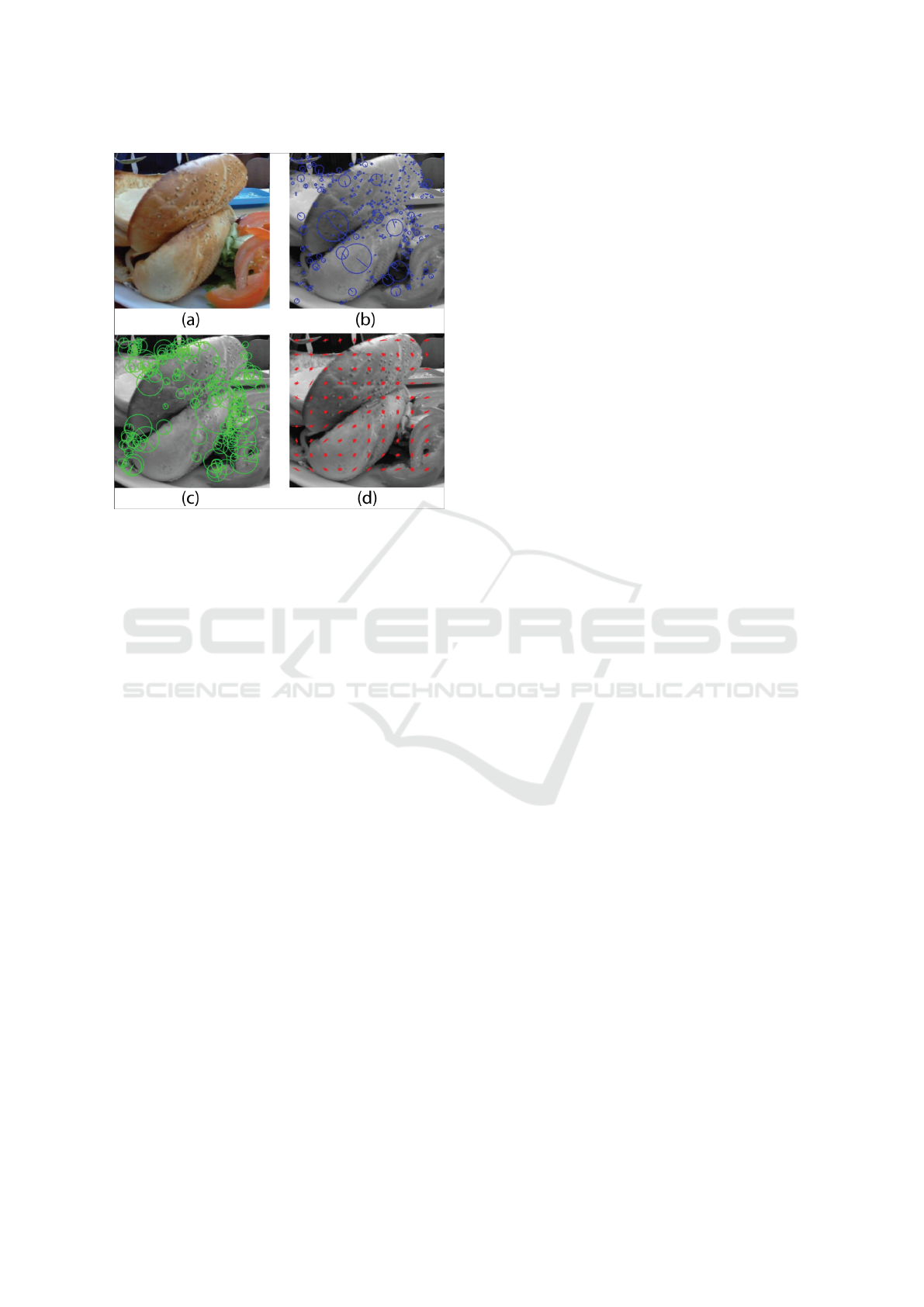
Figure 2: Feature selection. From the left to the right, the

top to the bottom: the original image, SURF features, SIFT

features and HOG features.

2.1 Hand-crafted Features

Recently, there have been many traditional features

that can be used in the object recognition prob-

lem. Among those, people usually use Scale Invari-

ant Feature Transform (SIFT) Lowe (2004), Speeded

Up Robust Features (SURF) Bay et al. (2006), and

Histograms of Oriented Gradients (HOG) Dalal and

Triggs (2005). All of these features are designed

to capture the characteristics of colors, textures and

shapes inside each object, which are then used for

classiﬁcation. However, each of these features has

its own pros and cons, and depending on the object

recognition problem, one has to choose the most ap-

propriate ones. Figure 2 illustrates an example of

these features.

SIFT, proposed by Lowe and colleagues, can ex-

tract a set of important key points in a given image.

It is interesting to emphasize that these key points

are mostly invariant with translation, scaling and ro-

tation. Normally, for computing SIFT features in an

image, one can do four following steps: scale-space

extrema detection by using the Difference of Gaussian

(DOG) matrix, key-point localizations, orientation as-

signment, and calculating key-point descriptors.

SURF, on the other hand, can be considered as a

fast version of the SIFT features. Instead of choosing

the DOG matrix to detect scale-space extrema, it cal-

culates an approximation of Laplacian of Gaussian by

Box Filters. Then, one can easily calculate each im-

age or all integral images for different scales by lever-

aging convolutions in box ﬁlters, wavelet responses in

orientation assignment and feature descriptors.

Additionally, HOG features are one of the most

well-known features for object recognition in the last

decade. To extract this feature from an image, one

needs to ﬁrst compute the gradient images by using

some ﬁlter kernels like 3 × 3 Sobel or diagonal ﬁl-

ters, and then calculates orientation binning by cell

histograms Bay et al. (2006). Finally, one can ex-

tract descriptor blocks from the left to the right and

from the top to the bottom, do block normalization,

and concatenate features in each block to create the

corresponding HOG features for the initial image.

For building a food recognition system, one can

use these local features to extract a feature vector for

each food image and then, with the corresponding la-

bels from training images, one can ﬁnd an appropriate

machine learning model for the system. This is the

traditional way for solving a classiﬁcation problem.

2.2 Convolutional Neural Networks

Convolutional neural networks are getting more

widely deployed for applications in computer vision

including object detection, object recognition and

video understanding. For a given input (an image) as

a 2D matrix of size N × N, all parameters of a CNN

are 2D ﬁlters of size m × m (m < N) which can be

convolved with all m × m sub-regions inside the im-

age followed by a nonlinearity to produce a tensor

output. By taking this advantage, each of these ﬁl-

ters only looks at one speciﬁc region of the input at a

time. For this reason, it can reduce the computational

cost of the traditional fully-connected networks where

each neuron connects to all of its inputs. Furthermore,

that makes CNNs suitable for any data such as images

where the spatial information is intrinsically local:

pixels at the top-left corner of an image may not be

related to the concept presented in the right-bottom.

Moreover, one can stack up multiple layers of con-

volutional ﬁlters followed by nonlinearities to make a

deep CNN architecture, where the ﬁrst layer extracts

features from the original image and the deeper layers

extract features from the shallower ones.

Recent experimental results Zeiler and Fergus

(2014) have shown that shallow ﬁlters usually help

in the extraction of low-level shapes (edges) while

deeper ﬁlters can extract higher and more abstract fea-

tures (faces or more complicated shapes). It turns out

that a deep CNN can be considered as a hierarchy of

ﬁlters which are learned to extract low to high level

features that are important to distinguish between dif-

ferent types of visual concepts. An illustration for

A Deep Learning based Food Recognition System for Lifelog Images

659

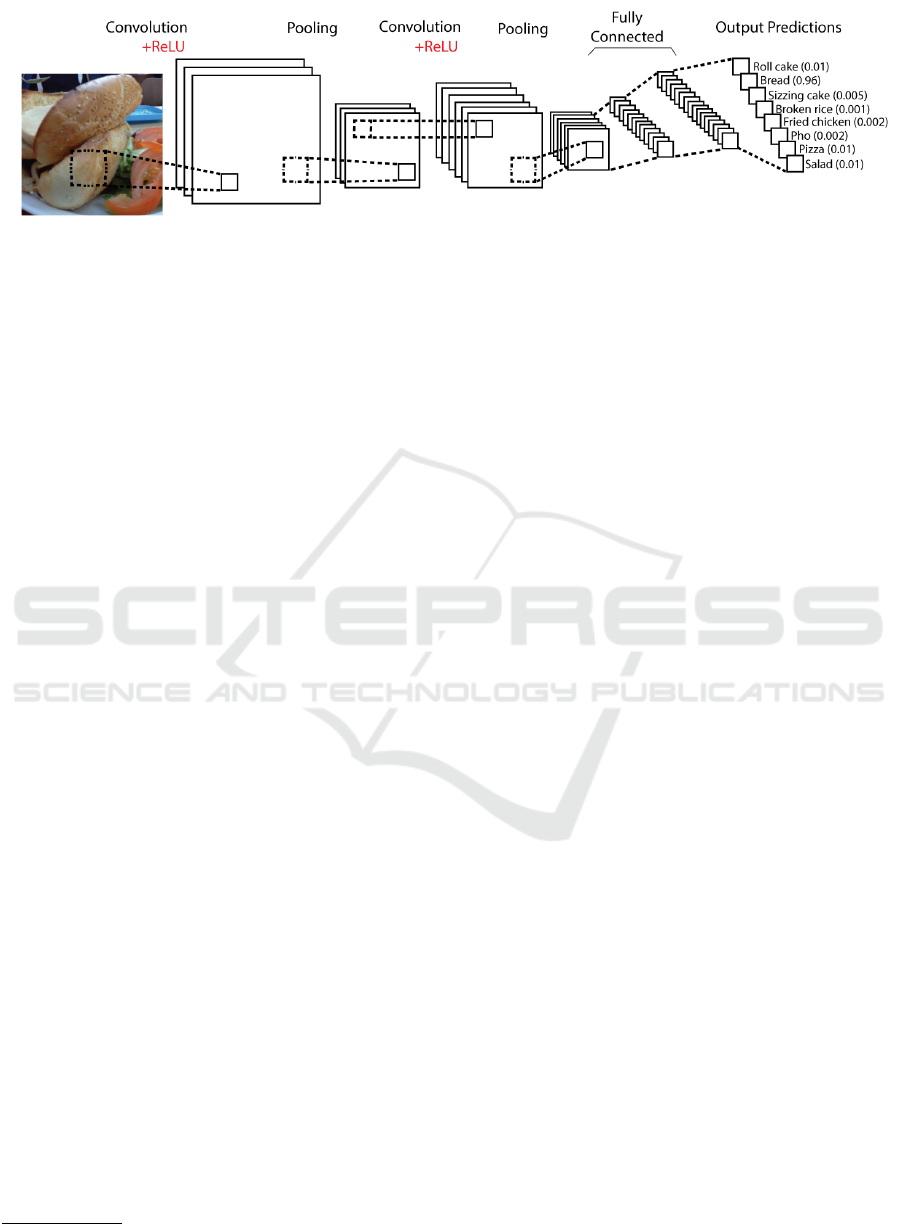
Figure 3: A proposed design of convolutional neural networks for food recognition from personal life archive images.

CNNs can be shown in Figure 3.

In this paper, we choose a transfer learning ap-

proach for classifying several types of foods from a

personal life archive of a lifelogger by choosing sev-

eral well-known architectures of CNNs and training

them on our own dataset. The ﬁrst architecture we

use is Alexnet Alex et al. (2012), the winner of the

ILSVRC

in 2012. This CNN contains ﬁve convolu-

tional layers, some of which are followed by max-

pooling layers and the classiﬁer is a 3 fully con-

nected layers with the ReLU activation function in

the ﬁrst two layers and the soft-max activation func-

tion in the ﬁnal one. The second model we choose

is GoogleNet Christian et al. (2015), the winner of

ILSVRC 2014. GoogleNet is an improved version of

Alexnet by replacing the large size ﬁlters in Alexnet

by inception module, a composition of submodules

including ﬁlters of different sizes as well as average

pooling. It is important to note that outputs of all sub-

modules are concatenated to create the ﬁnal output of

the whole module.

3 PRELIMINARY RESULTS

3.1 Dataset

As a preliminary experiment, we only test the last

module in the system: food recognition. To do so,

we exploit image collections from several lifeloggers,

and extract only food images (as many as possible)

from their personal life archives. Eventually, we built

a lifelogging food dataset that contains 14,760 images

of eight different foods: Vietnamese Roll Cake, Siz-

zling Cake, Broken Rice, Fried Chicken, Beef Noo-

dle, Bread, Salad, and Pizza. Each label has a number

of images varied from 2,000 to 3,000. These images

are manually annotated and labeled through an appli-

www.image-net.org/challenges/LSVRC/

cation written in Matlab. Some examples of the im-

ages are shown in Figure 4.

To perform experiments, we split the current

dataset into three sets: training set, validation set, and

testing set. For each food category, we randomly se-

lect 80% of images for training, 10% for validation,

and then use the remaining 10% of images for test-

ing. For each setting in the experiments, we create

an appropriate model from the training set and evalu-

ate the performance on the validation set. After that,

we choose the best snapshot which achieves the low-

est validation loss to evaluate the model on the test-

ing set. In our experiments, we have a brief compar-

ison among various hand-crafted features and archi-

tectures for CNNs.

3.2 Hand-crafted Features

One of important parts in our experiments is compar-

ing the performance of the proposed approach and the

collected dataset among different local features by us-

ing SIFT, SURF, and HOG. For each image, we re-

size it into a chosen size 200 × 200 pixels and extract

the corresponding features. For SIFT and SURF, we

compute all existent key-points and a descriptor ma-

trix with the default size N × 128 in which N is the

total key-points. It is important to mention that two

different images can have different numbers of key-

points (SIFT or SURF). However, the ﬁnal features

should have the same length. As a consequence, we

use Bag of Words to extract K words from the descrip-

tor matrix. It turns out that the ﬁnal feature vectors of

SIFT and SURF has the same length, K. For HOG, we

use the corresponding HOG extractors which are built

in our system and obtain the ﬁnal feature of length M.

For SIFT and SURF, we do a number of exper-

iments by choosing the total key-points varied from

100 to 300 and the number of words, K, between 10

and 40. For HOG, we select the cell size between

32 × 32 and 64 × 64, the block size from 2 to 6, and

the bin size between 9 and 18.

INDEED 2018 - Special Session on INsights DiscovEry from LifElog Data

660

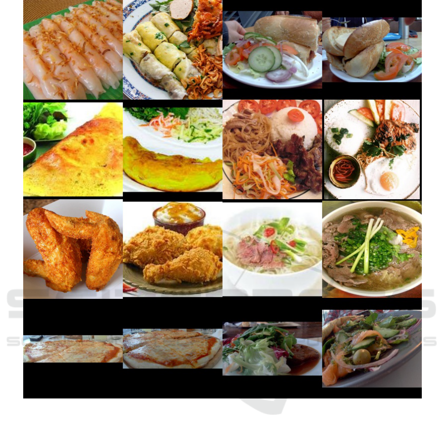
Figure 4: The lifelog food dataset with 8 different types of cuisines.

After computing the corresponding features

(SIFT, SURF, and HOG) in each image, we choose

appropriate classiﬁers by comparing two traditional

classiﬁcation approaches, SVM and XGBoost. Us-

ing the training/validation/testing dataset, we ﬁnd the

best parameters for each classiﬁer. More detailed, by

choosing various values for different parameters, we

train the corresponding models from the training data

and evaluate them on the validation set. Next, we se-

lect the best parameters having the best performance

on the validation set and check again on the testing

data.

In the experiments, we train SVM models by us-

ing different types of kernels, including linear, poly-

nomial, and RBF kernels. Detailedly, we choose γ

from 0 to 10, C from 0 to 10 and the degree of poly-

nomials from 2 to 5. For XGBoost, the number of

trees can be selected from 2 to 10 while the learning

rates are varied from 0.1 to 1 and the maximum depth

is chosen from 3 to 12. Finally, for implementation,

we use OpenCV libraries (version 2.4) for preprocess-

ing images and do computations for SIFT, SURF, and

HOG. For training and evaluating models, we utilize

all open libraries for SVM and XGBoost for building

the proposed system.

3.3 Convolutional Neural Networks

In this approach, we do a transfer learning step by

using architectures of two well-known convolutional

neural networks, AlexNet Alex et al. (2012) and

GoogleNet Christian et al. (2015), on our dataset. One

of main reasons we choose this approach is we would

like to see how these models work on our lifelogging

A Deep Learning based Food Recognition System for Lifelog Images

661

dataset. If they do not perform really well, we will

ﬁnd another architecture for CNNs.

To evaluate the performance of AlexNet and

GoogleNet, we ﬁrst resize an image into the size

227 × 227 for AlexNet Alex et al. (2012) and 224 ×

224 for GoogleNet Christian et al. (2015). For train-

ing these two CNNs, we use data augmentation and

dropout Nitish et al. (2014) with 80% probability to

reduce overﬁtting. For each batch of images, we gen-

erate new samples by randomly ﬂipping, rotation or

shifting on images with predeﬁned angles and dis-

tances. It is worth noting that we need to modify

the last fully connected layer in each model since the

number of categories in our problem is 8, completely

different from the total classes on the ImageNet data.

We aim at training two different versions for each

CNN: training-from-scratch (randomly initialized)

versus ﬁne-tuning (initialized with weights learned

from ImageNet). For training-from-scratch approach,

we normalize the input data by subtracting each im-

age with the mean RGB values which are computed

among the collected dataset, while for ﬁne-tuning ap-

proach, we use another mean RGB which are cal-

culated from ImageNet dataset. After normalization

step, we scale all data such that their standard devia-

tions are equal to 1. For training Alexnet and Google

Net, we choose the standard SGD optimizer with Nes-

terov accelerated gradient Botev et al. (2016) and mo-

mentum of 0.9. In addition, the batch size can be

selected as 64 for Alexnet and 32 for Google Net.

The learning rates can be selected in the following set

[0.0003, 0.001, 0.003, 0.01, 0.03]

3.4 Results

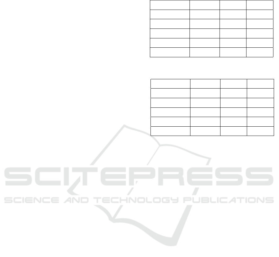
Table 1, Table 2, and Table 3 show the results ob-

tained by using hand-crafted features and CNNs, re-

spectively. In Table 1 and 2, we illustrate the perfor-

mance of using hand-crafted features (SIFT, SURF,

and HOG) and two different classiﬁers (SVM vs. XG-

Boost). There are ﬁve different features used in these

two tables: SIFT, SURF, HOG, and the combination

between two different features (HOG + SURF, HOG

+ SIFT). One can easily see that using SVM model,

HOG feature can achieve a better performance than

SIFT or SURF features. However, when one com-

bines HOG and SURF features to create a new fea-

ture, one can get the best accuracy (increasing the

accuracy from 51.28% to 60.08%). One can get the

same behavior when using XGBoost model. Finally,

using SVM models seems to achieve a better result

than XGBoost for these local features.

In Table 3, we describe the performance of top

3 settings above which achieve the highest accuracy

Table 1: Performance of different local features with SVM

models.

Method Train Set Val Set Test Set

HOG 92.87% 56.79% 51.28%

SIFT 58.33% 48.23% 45.77%

SURF 58.42% 51.77% 45.63%

HOG+SIFT 94.01% 64.20% 60.08%

HOG+SURF 93.65% 66.23% 59.47%

Table 2: Performance of different local features with XG-

Boost models.

Method Train Set Val Set Test Set

HOG 99.93% 46.81% 41.33%

SIFT 73.42% 45.58% 42.54%

SURF 76.94% 48.91% 44.49%

HOG+SIFT 89.18% 57.61% 49.66%

HOG+SURF 85.05% 54.07% 47.24%

on the validation set for each CNN model. The

experiments show that the ﬁne-tuning approach can

achieve a better convergence and performance than

the training-from-scratch approach. One possible rea-

son is all ﬁlters of CNNs can be pretty good for de-

tecting useful shapes for the object recognition prob-

lem when the dataset is large enough. In our work,

the number of images is 14,760, enough for building

a CNN. The performance of using GoogleNet is bet-

ter than the performance of Alexnet which is quite

expected.

According to these results, deep learning tech-

niques with the performance of 95.97% clearly out-

perform traditional hand-crafted features with the best

performance of 60.08%. Furthermore, we can ob-

serve an improvement of using GoogleNet instead

of AlexNet, by increasing the best accuracy from

91.67% to 95.97%. It is worth noting that these re-

sults are comparable to the results of the study in

Kawano and Yanai (2015) in which they obtained

92% classiﬁcation accuracy on the top-ﬁve on normal

food images.

4 DISCUSSION

The preliminary experiments were performed on the

assumption that the previous two steps of the pro-

posed system provide error-free results in detection of

food images from personal life archive. However, in

practice, that can be challenging as typical lifelogging

images do not only contain food images but rather

INDEED 2018 - Special Session on INsights DiscovEry from LifElog Data

662

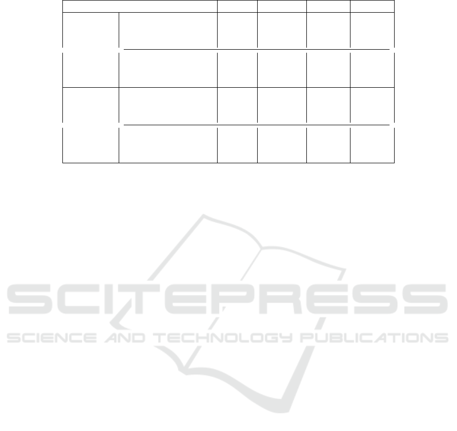
Table 3: Performance of GoogleNet and AlexNet.

Models lr Train Set Val Set Test Set

GoogleNet

ﬁne-tuning

0.0003 98.46% 95.38% 94.29%

0.001 99.93% 97.03% 95.97%

0.003 97.65% 93.71% 92.61%

training-from-scratch

0.0003 72.34% 73.73% 68.15%

0.001 78.82% 74.57% 72.72%

0.003 81.88% 77.88% 74.13%

AlexNet

ﬁne-tuning

0.0003 97.04% 93.01% 91.67%

0.001 96.21% 92.46% 91.53%

0.003 97.51% 89.74% 91.40%

training-from-scratch

0.0003 61.57% 62.23% 57.33%

0.001 63.21% 60.94% 57.93%

0.003 70.11% 70.11% 62.97%

they can reﬂect different objects and activities from

the lifelogger’s personal world. Thus, in the extended

version, the machine learning process must carefully

consider the outliers which are images that might con-

tain no food.

Further analysis in different scenarios should be

done, for example different light conditions or/and

different environments. Future work can also con-

sider utilising the system for other types of food, for

instance: the western food categories in NTCIR-12 -

Lifelog dataset Gurrin et al. (2016) and ImageCLE-

Flifelog 2017 Dang-Nguyen et al. (2017b) in Ionescu

et al. (2017).

5 CONCLUSION

In this paper, we have introduced the ﬁrst system for

recognizing food category of images from personal

life archive. We have compared different approaches

by using both hand-crafted features and CNNs. For

hand-crafted features, we have analyzed SIFT, SURF,

HOG, and the combination between SIFT + HOG

and SURF + HOG. After computing these local fea-

tures, we train appropriate models by using SVMs and

XGBoost. The experiments show that using HOG +

SIFT with SVM models can help us to achieve the

best performance with the accuracy 60.08% for the

ﬁrst approach. For the second approach, we have

used a transfer learning approach by utilizing AlexNet

and GoogleNet’s architectures for building a suitable

CNN model for lifelogging image dataset. The ﬁ-

nal experiments show that using GoogleNet architec-

ture but modifying the last fully-connected layer can

help us to achieve the best model for this problem

with the highest accuracy 95.97% for 8-label classi-

ﬁcation. Future work should evaluate the system on

bigger datasets and in more challenging scenarios.

6 ACKNOWLEDGEMENT

We would like to thank to Dr. Zaher Hinbarji from

Dublin City University and Mr. Quang Pham from

Singapore Management University for their valuable

discussions and technical supports.

REFERENCES

A., T. (1992). Monitoring food intake in europe: a food data

bank based on household budget surveys. European

journal of clinical nutrition.

Alex, K., Ilya, S., and Geoffrey, E., H. (2012). Im-

agenet classiﬁcation with deep convolutional neural

networks. NIPS.

Bay, H., Tuytelaars, T., and Van Gool, L. (2006).

SURF: Speeded Up Robust Features, pages 404–417.

Springer Berlin Heidelberg, Berlin, Heidelberg.

Botev, A., Lever, G., and Barber, D. (2016). Nesterov’s Ac-

celerated Gradient and Momentum as approximations

to Regularised Update Descent. ArXiv e-prints.

Christian, S., Wei, L., Yangqing, J., Pierre, S., Scott, R.,

Dragomir, A., Dumitru, E., Vincent, V., and Rabi-

novich, A. (2015). Going deeper with convolutions.

Proceedings of the IEEE.

Dalal, N. and Triggs, B. (2005). Histograms of oriented gra-

dients for human detection. In 2005 IEEE Computer

Society Conference on Computer Vision and Pattern

Recognition (CVPR’05), volume 1, pages 886–893

vol. 1.

Dang-Nguyen, D.-T., Zhou, L., Gupta, R., Riegler, M.,

and Gurrin, C. (2017a). Building a disclosed

lifelog dataset: Challenges, principles and processes.

In Proceedings of the 15th International Workshop

on Content-Based Multimedia Indexing, CBMI ’17,

pages 22:1–22:6, New York, NY, USA. ACM.

A Deep Learning based Food Recognition System for Lifelog Images

663

Dang-Nguyen, Duc-Tien, P. L., Riegler, M., Boato, G.,

Zhou, L., and Gurrin, C. (2017b). Overview of image-

cleﬂifelog 2017: Lifelog retrieval and summarization.

CEUR-WS.org.

Ge, Z., McCool, C., Sanderson, C., and Corke, P. I. (2015).

Modelling local deep convolutional neural network

features to improve ﬁne-grained image classiﬁcation.

CoRR, abs/1502.07802.

Gurrin, C., Albatal, R., Joho, H., and Ishii, K. (2014a). A

privacy by design approach to lifelogging. Digital En-

lightenment Yearbook 2014, pages 49–73.

Gurrin, C., Joho, H., Hopfgartner, F., Zhou, L., and Albatal,

R. (2016). Overview of NTCIR-12 Lifelog Task.

Gurrin, C., Smeaton, A. F., and Doherty, A. R. (2014b).

Lifelogging: Personal big data. Foundations and

Trends in Information Retrieval, 8(1):1–125.

Ionescu, B., M

uller, H., Villegas, M., Arenas, H., Boato, G.,

Dang-Nguyen, D.-T., Dicente Cid, Y., Eickhoff, C.,

Seco de Herrera, A. G., Gurrin, C., Islam, B., Kovalev,

V., Liauchuk, V., Mothe, J., Piras, L., Riegler, M., and

Schwall, I. (2017). Overview of ImageCLEF 2017:

Information Extraction from Images, pages 315–337.

Springer International Publishing, Cham.

Kawano, Y. and Yanai, K. (2015). Foodcam: A real-time

food recognition system on a smartphone. Multimedia

Tools Appl., 74(14):5263–5287.

Liu, J., Johns, E., Atallah, L., Pettitt, C., Lo, B., Frost, G.,

and Yang, G.-Z. (2012). An intelligent food-intake

monitoring system using wearable sensors. In Pro-

ceedings of the 2012 Ninth International Conference

on Wearable and Implantable Body Sensor Networks,

BSN ’12, pages 154–160, Washington, DC, USA.

IEEE Computer Society.

Lowe, D. G. (2004). Distinctive image features from scale-

invariant keypoints. International Journal of Com-

puter Vision, 60(2):91–110.

Lukas, B., Matthieu, G., and Luc, Van, G. (2014). Food-

101 - mining discriminative components with random

forests. Springer.

Nitish, S., Alex, K., Ilya, S., and Geoffrey, E., H. (2014).

Dropout: A simple way to prevent neural networks

from overﬁtting. JMLR.

Pizer, S. M., Amburn, E. P., Austin, J. D., Cromartie, R.,

Geselowitz, A., Greer, T., Romeny, B. T. H., and Zim-

merman, J. B. (1987). Adaptive histogram equaliza-

tion and its variations. Comput. Vision Graph. Image

Process., 39(3):355–368.

Yoshiyuki, K. and Keiji, Y. (2014). Food image recognition

with deep convolutional features. ACM.

Zeiler, M. D. and Fergus, R. (2014). Visualizing and Un-

derstanding Convolutional Networks, pages 818–833.

Springer International Publishing, Cham.

Zhou, L., Dang-Nguyen, D.-T., and Gurrin, C. (2017). A

baseline search engine for personal life archives. In

Proceedings of the 2nd Workshop on Lifelogging Tools

and Applications, LTA ’17, pages 21–24, New York,

NY, USA. ACM.

INDEED 2018 - Special Session on INsights DiscovEry from LifElog Data

664