Predicting Cognitive Impairments with a Mobile Application

Elif Eyig¨oz, Guillermo Cecchi and Ravi Tejwani

IBM Research, Yorktown Heights, NY, 10598, U.S.A.

Keywords:

Automatic Prediction of MMSE, Syntactic Complexity, Cognitive Impairments.

Abstract:

Assessment of cognitive impairments is of social and clinical importance for vulnerable populations, such as

elderly, athletes and soldiers, who are prone to falling victim to cognitive impairments. This paper presents

ongoing work for developing an application that predicts the neurological state of users with the state-of-

the art performance through analyzing the structural complexity of users’ utterances. We present a novel

method that estimates the neurological state of users with Pearson correlation of 0.66 with respect to the

Mini-mental state exam score. Unlike previous work, our method does not depend on assumptions of relating

linguistics representations to human language-processing capabilities, but discovers the discriminative patterns

automatically.

1 INTRODUCTION AND

MOTIVATION

In this p aper, we present ongoing work on develop-

ment of a mobile application that estimates the degree

of cognitive im pairment of a user with state-of-the-

art performance, upon co llec ting a speech sample by

prompting the user with a picture description task. We

expect a large portio n of our users to be people with

cognitive impairments due to aging related neurode-

generative disorders, and people with traumatic brain

injury.

Dementia is a growing social and clinical pro-

blem, as three percent of people between the ages

of 65 and 74, 19% between 75 an d 84, and nearly

half of those over 85 have the condition (Umphred,

2007). Early detection of the disorder, coupled with

access to care planning leads to better outcomes for

both patients and their caregivers (Bradford et al.,

2009). The true prevalence of missed and de la yed

diagnoses of dementia is unkn own but seems to be

very high (Bradford et al., 2009). Diagnosis of de-

mentia is prone to be delayed, because it is dependent

on suspicion and concern based on patients symp-

toms. A major factor for delayed diagnosis is lack of

access to affordable healthcare, as patients in lower

strata tend to go undiagnosed at a higher rate (Ma-

estre, 2012). Accordingly, economic issues are also

critical for control and management of dementia af-

ter diagnosis. Therefore, cost-effective, easy-to-use

and naturalistic tools for routine dementia-screening

and disease-progression monitoring c ould provide pa-

tients and medical profe ssionals with the oppo rtunity

to engage in efﬁcient tr eatment planning.

Our tool is going to be useful for assessing not

only slow-developing cognitive impairments like de-

mentia, but also for sudden changes in cognitive ca-

pabilities, for example due to a traumatic brain in-

jury (TBI), or a stroke. In 2013, about 2.8 m illion

TBI-related emergen cy department visits, hospitaliza-

tions, and deaths oc curred in the United States (Sosin

et al., 19 96). Mem bers of certain professions, such as

athletes and c ombat soldiers, are more prone to falling

victim to TBI (Cole et al., 2017). Currently, there are

several computerize d neuroc ognitive assessment tests

used for TBI that engage various cognitive domains,

such as m emory, attention, motor speed, processing

speed etc. (Cole et al., 2017). However, none of these

tests perform language analysis using NLP techno-

logy with linguistic sophistication that can quantify

structural complexity of a speakers utterances. There-

fore, o ur to ol is going to be a signiﬁcant contribution

to the existing battery of computerized neurocognitive

assessment tools used for TBI.

In this paper, we present a novel method for esti-

mating the degree o f cognitive imp a irment, and also

describe our efforts o n building a prototype. We vali-

date our method by p erforming regression to predict

the Mini-Mental State Examination (MMSE) score.

MMSE is a neuropsycholog ic al test that is used exten-

sively in clinical resear ch to estimate the severity a nd

progression of cognitive impairment (Folstein et al.,

Eyigöz, E., Cecchi, G. and Tejwani, R.

Predicting Cognitive Impairments with a Mobile Application.

DOI: 10.5220/0006734006830692

In Proceedings of the 10th International Conference on Agents and Artiﬁcial Intelligence (ICAART 2018) - Volume 2, pages 683-692

ISBN: 978-989-758-275-2

683

1975; Pangman et al., 2000). I t is the best studied

and the most commonly used test for the diagnosis

and longitudinal assessment of Alzheimer’s Disease -

the most common type of dementia (Burns and Iliffe,

2009). MMSE is also considered as an effective way

to document an individual’s respo nse to treatment

(Pangman et al., 2000). MMSE is also used for eva-

luating cognitive o utcome in patients with TBI, both

immediately following an inju ry and in the follow-up

period, although its sensitivity de pends on the site of

injury (Lee et al., 2015; De Guise et al. , 2013).

We u se NLP techniques, in particular syntactic

analysis of constituent pa rse trees for feature ex-

traction. To validate our method, we used data

from the Pitt Corpus, whic h is part of the publicly

available DementiaBank corpus (Macwhinney et al.,

2011). Our method can successfully estimate the cog-

nitive impairment of subjects in the DementiaBank

study with Pearson correlation of 0.66 with respect

to MMSE, which is currently the state-of-the art in

predicting MMSE.

The outline of the paper is as follows: We ﬁrst

summarize related work in Sectio n 1.1; we then pro-

vide necessary background for presenting our f eature-

extraction method in Section 2, present th e feature-

extraction method for predicting MMSE in Section 3,

and the feature-selection method in Section 4; we dis-

cuss the per formanc e of our method in Section 6, and

describe the current status of our implemen ta tion and

future development plans in Section 7.

1.1 Related Work

There is growing number of papers in the recent ye-

ars using the DementiaBank corpus, predominantly

doing classiﬁcation of patients vs hea lth controls (Fr a-

ser and Hirst, 2016; Fraser et al., 2016; Orimaye et al.,

2014, 2017). Fraser et al. (2016) use syntactic, se-

mantic, lexical and acoustic features to classify Alz-

heimer’s disease patients vs healthy controls in De-

mentiaBank. They used context free gr a mmar (CFG)

rule rates and proportions in sample interviews as fe-

atures, in addition to average length of the r ight hand

side of CFG rules, only for noun phrases (NP), verb

phrases (VP), and prepositional phrases (PP). They

obtained 81 percent classiﬁcation accuracy, how ever

the results they re ported were obtained with featu-

res that were selected using the entire data set. Ori-

maye et al. (2014) and Orimaye et al. (2017) also

used syntactic f eatures for classiﬁcation of Alzhei-

mer’s disease patients vs healthy controls in Demen-

tiaBank. They used syn ta ctic features involving sen-

tence embeddedness, in particular they focused on

POS tags indicating coordinated, subordinated, and

reduced sentences ( CC, S, VBG, V BN). They also

used counts of unique CFG rules, the valency of

verbs, lexical features involving repetition. Their re-

sults were also obtained using features that were se-

lected using the e ntire data set.

To the best of our knowledge, the only study that

predicted MMSE scores using linguistic features is

Ya ncheva et al. (2 015), where they modele d longitu-

dinal progression of MMSE scores using su bjects that

have more than o ne sample in DementiaBank. They

reported a mean-a bsolute-err or (MAE) of 2.91 in pre -

dicting MMSE , signiﬁcantly below the within-subject

inter-rater standard deviation of 3.9 to 4.8 (Molloy

et al., 1991). However, the lowest MAE they obtained

with a method generalizable to unseen data was 7.31,

as they also reported results obtained with using fea-

tures that were selected using the entire data set. They

did not report the correlation between the scores their

method predicted and the actual MMSE scores.

Our work differs from m ost psycho linguistics and

neuroscience studies on linguistic aspects of neurolo-

gical disorders in multiple ways: First and foremost,

our method is not intended f or theore tical understan-

ding of h uman language production and processing

capabilities, but for practical application s.

Second, we present results that are g eneralizable

to unseen data. We perform feature-selection in each

cross-validation (CV) fold separately without obser-

ving the entire data set, and use all f eatures selected

in the folds of CV, as opposed to related work that re-

port results obtained with features selected using the

entire data set.

Finally, a major difference between related work

and our method is that out method does not depend

on assumptions relating linguistics representations to

human-language-processing capabilities. Prior stu-

dies all use hand written rules involving node labels

(e.g. NP, VP, S), naturally supported by the psycholo-

gists literature, for feature extraction. Our method, on

the other hand, do es not depend on the actual syntax-

tree labels. For example, the tree in Figu re 1(a) has

node lab els that a re commonly used in language stu-

dies, however the trees in Figure 1(b) have node labels

that are variables. Our method can be used on either

types of trees, and thus can b e applied to trees of any

syntactic theory, as long as we can obtain parse trees

of utterances for training and testing. A major advan-

tage of this approach is that we can, an d do, apply our

method to la nguages other than E nglish, which do not

use familiar node labels.

NLPinAI 2018 - Special Session on Natural Language Processing in Artiﬁcial Intelligence

684

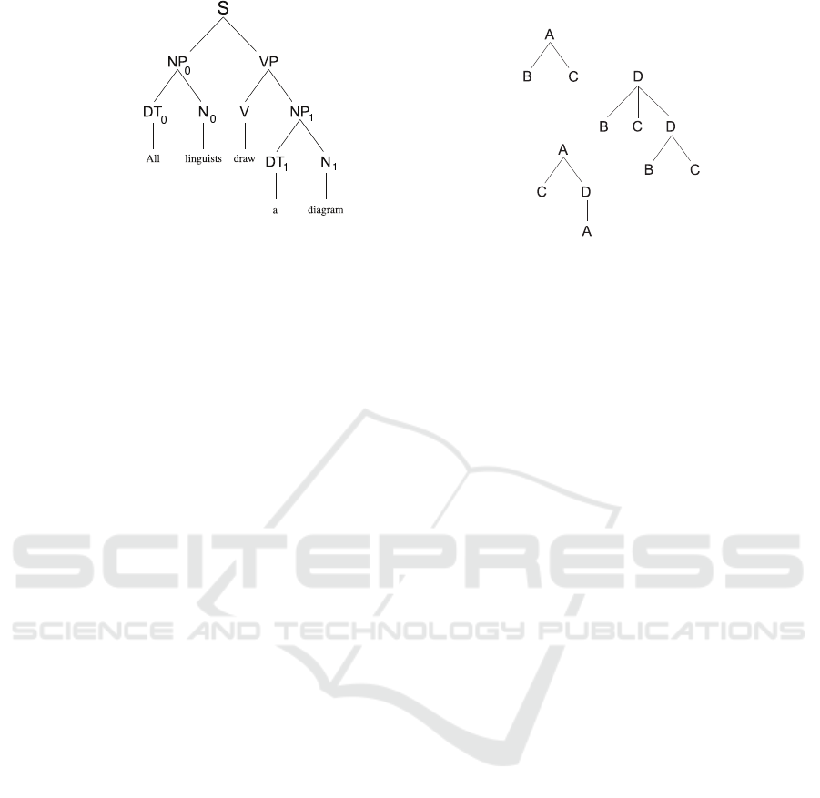
(a) (b)

Figure 1: Example syntax trees.

2 BACKGROUND

2.1 Syntax Trees

We model the stru ctural complexity of users’ utteran-

ces through syntactic analysis. In particular, we ana-

lyze constituency parse of the utterances, which are

obtained by a statistical p arser. In this section, we de-

ﬁne basic syntactic tre e relations in order to provide a

backgr ound for our feature extraction meth od.

Figure 1(a) shows a constituency parse for the sen-

tence “All linguists draw a diagram”. As shown in Fi-

gure 1(a), parse trees are graphs that are made up of

nodes (e.g. NP, VP), and edges that connect the nod es.

Nodes have labels, such a s NP for a noun phrase, VP

for a verb phrase etc. The node labels in this study fol-

low the convention of constituent tags in Penn Tr e e-

bank (Marcus et al., 1993), as we used a statistical

parser trained on Penn Tree bank to parse our data.

However, our method does not depend on having prior

knowledge of actual node la bels, as we could have

used some other method, and obtained trees with a

different label set, for example if we apply our met-

hod to another langua ge.

Nodes NP

and NP

have the same label, NP, as

the subscripts are not parts of the node labels. We use

the subscripts, e. g. NP

, on the labels in Figure 1(a)

for disambiguation between the nodes with the same

label. Branch out o f a tre e node is conveyed in a con-

text free grammar (CFG) rule, for example as ‘NP →

DT N’, whic h is instantiated twice in Figure 1(a): NP

that branches to DT

and N

, and NP

that branches

to DT

and N

. A CFG rule covers all and only the

nodes that branch out of a sing le no de. Our work dif-

fers from related work using syntax, in that they mos-

tly use CFG rules, but not sm aller or larger subtree

patterns.

In the deﬁnition s of this paper, we assume trees

have only directed edges, in that the nod e s can be tra-

versed throu gh the edges only in a top down fashion.

For example, there exists a path to all nodes in the tree

from node S, however there is no path that can re a ch

node S, as it is at the top of the tree and nodes can be

traversed only in a top down fashion. For this reason,

node S is called the root of the tree, and syntax trees

have a single root node. Th e tree under the root node

covers the entire sentence, whereas trees under other

nodes span subparts of the sentence. Fo r example, the

tree u nder the node with label VP spans “draw a dia-

gram”. The subspan covered by a node is called the

yield of that node. In Figure 1(a), there are two NPs,

one has the yield “all linguists”, and the other has the

yield “a diagram”. Some nodes have yields that are

only single words. For example, the no de with label

yields only the word “diagram”.

2.2 Relations between Nodes

In this section, we deﬁne tr ee relations that span smal-

ler and larger subtr ees than CFG rules. The most pri-

mitive relations between nodes in a tree are mother,

sister, dominance r elations. Node a dominates node

b, if and only if (iff ) there is a path betwee n the root

node and b which passes through a. For example, NP

dominates DT

, and VP dominates N

. Node a is th e

mother of nod e b, iff a dominates b, and there is an

edge between a and b. For example, node NP

is th e

mother of node DT

. Node a is a sister of node b, iff

they have the same mother. For example, node DT

and node N

are sisters.

The root node S in Figure 1(a) dominates DT

and the path be twe en them has three edges. There-

fore, the domina nce relation can have a larger scope

than CFG rules, which can only represent relatio ns of

depth one. For feature extraction, we use dominance

relations between nodes that are two edges apart.

Predicting Cognitive Impairments with a Mobile Application

685

In addition, we make use of tre e relations with

larger scope than CFG rules that were ﬁrst deﬁned

within the Chomskyan tradition. The ﬁrst rule is c-

command (Haegeman, 1994) . Within the sco pe of this

paper, c-command b etween two nodes could be des-

cribed informally a s an aunt relation, if we contin ue

with the analogy of sisterhood and motherhood as re-

lations b etween nodes. Formally, c-command is deﬁ-

ned as follows: node a c-commands node b, iff a does

not dominate b, b does not dominate a, and the lo-

west branchin g nod e c tha t dominates a dominates b.

For example in Figure 1(a), node V c-commands N

-i.e. V is the aunt of N

- because V does not domi-

nate N

, N

does not dominate V, and VP is the mot-

her of V, which dominates N

. The formally-deﬁned

c-command r elation can span nodes of arbitrary dis-

tance. However, we limit our feature-extrac tion met-

hod to consider only the most local c-command re-

lations, which c a n informally be deﬁned as aunt re-

lations. According to the formal deﬁnition, sister re-

lation is also a c-command-relation. Howeve r, we do

not consider sister relations as c-command relations in

this paper, as we alread y use sister relations for fea-

ture extraction, and want to keep c-command and sis-

ter relations mutually exclusive for feature extraction.

Next, w e deﬁne a terna ry version of the c-

command relation: c-command is deﬁned between

two nodes, a and b, whereas c-command-via-node

is deﬁned not only between a and b, but also in-

cludes c, where node c could be deﬁned informally

as the grandmother of node b. Formally, node a c-

commands b via c, iff a does not dominate b, b does

not dominate a, an d the lowest branching n ode c that

dominates a dominate s b. For example in Figure 1(a),

node V c-commands N

via VP. Within the scope of

this paper, this relation is constrained to cover only

ternary relations that exists between a nod e, the no-

des aunt, and the nodes gra ndmoth e r, as deﬁned in-

formally.

Finally, we also use a ternary dominate-via-node

relation, that includes a node , the nodes mother, and

the nodes grandmother, w here a node is dominated

by its g randmo ther via its mother. To summ arize,

we use the following relations for f e ature extraction:

sister, dominate, c-command, c-command- via-nod e,

dominate-via-node, and the nod e labels.

3 FEATURE EXTRACTION

3.1 Subtree Patterns

We illustrate our metho d of feature extraction with the

example trees in Figu re 1(b ). There are multiple trees

in Figure 1(b), as most samples consist of multiple

utterances. In the example, the node labels are not

from the Penn-Treebank constituent tag set. Instead,

we used variables for node labels in the example, ﬁrst

to empha size that our method do es no t dep end on the

actual node labels, but their relations in the trees, as

deﬁned in Section 2. Second, because it is common to

use variables for node labels for generalizability, and

also for easy-readability.

Table 1 lists instances of node labels, sister rela-

tions, and c-command-via-node relations observed in

the trees in Figure 1(b), and their counts. Let us ﬁrst

look at the examples of node labels in the ﬁrst column

in Table 1. Tota l number of nodes in the trees in Fi-

gure 1(b) is given in the last row. We divide the count

of a node label by the total count of nodes. For ex-

ample in Figure 1(b), there are three nodes labeled as

B, and the total count of nodes is 13. Thus th e rate of

nodes labeled B is 3 /13.

In the second column in Table 1, we show counts

of sister relations in the trees in Figure 1(b). We ob-

serve node B and C as sisters three times, C and D as

sisters two times, B and D as sisters only once . For

each sister relation instance, w e divide the count of

that instance by the total number of sister relations.

For example in Figur e 1(b), the count of sister(B,C)

is three , the total count of sister relation s is six. Thus,

the rate of sister(B,C) is 3/6. Th e counts of all sister

relation instanc es, and the total count of sister relati-

ons are shown in Table 1. In sum, a rate is obtained

for each instance of the sister relation by dividing the

count of that instance by the sum of the counts of all

instances of the sister re la tion.

Similarly, the rates of instances of the c-

command-via-node relation are co mputed in the same

manner, as shown in Table 1. For all relations menti-

oned in the previous section, we obtain a rate for each

instance of the relation by dividing the count of that

instance by the sum of the coun ts of all instances of

that relation. We use logarithm of the rates as featu-

res, and use 10e-7 as ﬂoor in order to avoid computing

the logarithm of zero.

Finally, we also use features involving CFG rules:

We normalize the counts of instance s of CFG rules

by the total number of CFG rules in a sample. For

example, the CFG rule A →B C occu rs only onc e in

Figure 1(b), and there are total ﬁve CFG rules in Fi-

gure 1(b), thus the rate of A →B C is 1/5. We also use

statistics over the le ngth of CFG rules -as the num-

ber of nodes at the right side of CFG rules- in a sam-

ple. We compute minimum, maximum, mean, stan-

dard deviation and percentiles over the length of CFG

rules as features.

NLPinAI 2018 - Special Session on Natural Language Processing in Artiﬁcial Intelligence

686

Table 1: Example counts of subtree patterns.

Unary Binary Ternary

Node-label Count Rate Sister Count Rate C-command-via-node Count Rate

A 3 3/13 Sister(B,C) 3 3/6 Comm-max(B,B,D) 1 1/5

B 3 3/13 Sister(C,D) 2 2/6 Comm-max(B,C,D) 1 1/5

C 4 4/13 Sister(B,D) 1 1/6 Comm-max(C,B,D) 1 1/5

D 3 3/13 Comm-max(C,C,D) 1 1/5

Comm-max(C,A,A) 1 1/5

Node total 13 Sister total 6 Comm-max total 5

3.2 Node Scores

Statistical parsing algorithms compute a score bet-

ween 0 and 1 for each node, indicating how gram-

matical the yield of a node is within the context o f

the entire sentence. We obtain the node scores from

the statistical parsers data structures. For each node

label, we compute statistics over the scores assign e d

to the nodes with that label in the sample. We com-

pute maximum, minimum, standa rd deviation, skew-

ness and kurtosis over the node scores for each label,

and use them as features.

4 FEATURE-SELECTION

METHODS

As we do not assume prior knowledge of what node

labels o r subtr ee patterns indicate in terms of syn-

tactic comp lexity with respect to human language

processing, we generate a large number of features

for all observed subtree patterns in the samples. As

a res==ult, eliminating features of low quality is es-

sential to th e performance of our method. We re-

sorted to an experimental method for e liminating low

quality features within a leave-one-subject-out cross-

validation setting (LOOCV). We split the data to folds

of train-test sets. Within each fold, we performed

feature-selection as exp la ined below, and predicted

the scores of the samples from the left-out-subject

using the selected features.

Univariate Feature Selection. As initial ﬁltering,

we used univariate feature selection methods. We

obtained a p-value for each feature by computing

Pearson r between the feature and the MMSE sco-

res. We eliminated features with p-value greater than

0.01. Then, we performed an ANOVA-F test, and mo-

deled the decreasing p-values as an exponential-decay

curve. We used curve ﬁtting to obtain the τ parameter

for the decay curve. We learned a multiplier a for the

τ parameter with cross-validation, w here α· τ is u sed

as a thresh old to eliminate features that are at the tail

of the exponential-d ecay curve.

Stability-selection. We followed univar ia te

selection methods with stability-selection (Meins-

hausen and B¨uhlmann, 2010). We used the

scikit-learn

implementation of Randomized

Lasso, which returns a score for each feature.

We modeled the decreasing feature scores as an

exponential-decay curve. We used curve ﬁtting to

obtain the τ parameter, and learned a multiplier a for

the τ par ameter with cross-validation, where α · τ is

used as a threshold to eliminate features that are at

the tail of the exponential-de cay curve.

Recursive-feature-elimination. Next, we used re-

cursive feature elimination (RFE). Given an estima-

tor, RFE selects features by recursively consider ing

smaller and smaller sets of features. First, the estima-

tor is trained on the initial set of features and weig-

hts are assigned to each one of them. Then, featu-

res whose absolute weights are smallest are pruned

from the curr ent set features. This procedure is recur-

sively perfor med on the pruned set until the features

are exhausted.

RFECV

in the

scikit-learn

package performs

RFE in a cross-validation loop to ﬁnd the optimal

set of features.

RFECV

requires an estimator to obtain

weights for the features, for which we used Linear Re-

gression. As

RFECV

returns an optimal set of features,

we rer un

RFECV

using the optimal set returned by the

previous run, until it no longer retur ned a smaller set.

In other words, we repe ated

RFECV

until it conve rged.

Feature-selection in LOOCV. Within each fold of

LOOCV, we started with univariate f eature-selection

Predicting Cognitive Impairments with a Mobile Application

687

methods, as they can quickly eliminate a large number

of features of low statistical signiﬁcance. Eliminating

large numb er of fe atures is critical for subsequent fea-

ture selection methods, namely stability-selection an d

recursive-feature-elimination, as they can be a lot slo-

wer than the univariate feature-selection methods.

Recursive-feature-elimination, unlike stability-

selection, can be unstable across folds in terms of

the number of features it eliminates. For that rea-

son, we perform stability-selection before recursive-

feature-elimination. Performing recursive-feature-

elimination as the last step of feature-selection ensu-

res that it evaluates only a small number of features

in each fold, thus the instability of the method can be

relatively constrained.

Finally, the selected fea tures in each fold were

used for training, and the scores of the test sam ples

were predicted using the ﬁtted estimato rs.

5 DATA

We validated the f e ature extraction method explain ed

in the previous section for prediction of MM SE using

the publicly available DementiaBank corpus (Macw-

hinney et al., 2011). Patients of various types of

dementia were included in the study, in addition to

age and education matched healthy controls. Demo-

graphics of DementiaBank can be found in Table 2.

All subjects were given the Cookie Theft picture

description task from the Boston Diagnostic Aphasia

Examination (Kaplan, 1983). Th is task was chosen,

because it is considered an e cologically valid approx-

imation to spontaneous discourse. We used each nar-

rative for the description a s a sample, and parsed the

utterances using the Stanford Parser (Klein and Man-

ning, 2003). All subjects were associated with a pro-

fessionally administered MMSE score on a scale of

0 (greatest cognitive impairment) to 30 (no co gnitive

impairment).

Table 2: DementiaBank Demographics.

Dementia Control

Number of sample s 278 182

Number of subjects 192 96

Age (years) 72 (8.66 ) 64 (7.48 )

Gender (male/female) 101/177 66/115

MMSE 20 (5.7) 29 (1.1)

Table 3: Feature-selection results for the baseline model,

which uses only features involving CFG rules, and the best

performing model, which uses all subtree patterns. The

second column shows t he median number of features se-

lected across folds by the method given in t he ﬁrst column.

The feature-selection methods are listed sequentially with

respect to their application.

(a) CFG Rule s

Total # Features 978 Pearson r MAE

1 Pearson r <0.01 65 0.60 4.08

2 ANOVA f-test 20 0.61 3.94

3 Stability 18 0.61 3.93

4 RFE 16 0.60 3.95

(b) Subtree patterns.

Total # Features 4297 Pearson r M A E

1 Pearson r <0.01 468 0.62 3.97

2 ANOVA f-test 99 0.66 3.86

3 Stability 35 0.64 3.91

4 RFE 35 0.64 3.91

6 EXPERIMENTS AND RESULTS

Features involving CFG rules were comm only used

in previous work for classiﬁcation of patien ts vs con-

trols in DementiaBank . Th e refore, we use features

involving CFG rules as a baseline model. Please note

that we used all CFG rule s observed in the interviews,

not only CFG rules involving a pre-determined set of

node labels. We have in total three experimental con-

ditions:

• Baseline: CFG features

• All subtree patterns: CFG features plus features

involving other subtree pa tterns, e.g. sister, domi-

nance, and c-command relations, as explained in

Section 3.1.

• Node scores: As explained in Section 3.2.

Table 3 shows the results obtained after each

feature-selection step for e ach experimental condi-

tion. We do not report these detailed feature-selection

results for the node scores experiment, as it was the

worst performing experimental condition, as shown

in Ta ble 4. It shows the sequential decrease in the

number of features after each feature-selection step.

In both experiment conditions, the largest decrease

in the number of features was obtained by the ﬁrst

feature-selection step, and the smallest decrease in the

NLPinAI 2018 - Special Session on Natural Language Processing in Artiﬁcial Intelligence

688

Table 4: The best estimators.

Subtree patterns CFG rules Node scores

# Features 35 16 34

Pearson r 0.64 0.60 0.56

Estimator Lasso CD All Ridge CD

MAE 3.91 3.95 4.29

Estimator Ridge / Elastic Net eSVR Linear Regression

number of features was obtained by the last feature-

selection step . In Table 3, we report results obtained

with the selected feature s in terms of Pearson r cor-

relation between th e predicted scores, and the actual

MMSE scores. In addition, we report mean-absolute-

error (MAE) between the predicted scores and the

actual MMSE scor es. Although MAE is a scale-

dependent measu re, we have to report results with this

metric, as previous results on predicting MMSE sco-

res both au tomatically and manually have be e n repor-

ted in terms of MAE.

Table 4 shows the best perfor ming estimators on

the sm allest number o f fea tures after all feature-

selection steps had been applied. In Tab le 4, the

ﬁrst row shows the experimental conditions, the se-

cond row shows the median number of features se-

lected across folds per experimental condition. The

row for Pearson r shows the correlation b e tween the

predicted MMSE scores and the ac tual MMSE sco-

res. The next row shows the estimator that obtained

the Pear son r performance. The MAE row shows the

mean-ab solute-erro r between the predicted MMSE

scores and the actual M MSE scores. The row under

the MAE row shows the estimators that obtained the

MAE perform ance. The com plete list of estimators

we ex perimented with, along with their initialization

and grid search parameters can be found in the Ap-

pendix. In Ta ble 4, “All” stands for all estimators gi-

ven in the Appendix.

6.1 Discussion

The highest correlation for pre diction of MMSE was

obtained by using all subtree pattern s, with Pearson r

of 0.66, as shown in Table 3(b). The improvement in

Pearson r over the baseline, as shown in in Table 3(a),

was ﬁve percent. Therefore, using subtree patterns

that have smaller scope than CFG ru les, such as sister

relations, and subtree patterns that have larger scope

than CFG rules, such as c-command relations, impro-

ved performance.

Table 3(b) shows that, the performance was op-

timal after using only the ﬁrst two feature-selection

steps: using a p -value threshold and the ANOVA f-

test. Howeve r, stability-selection resulted in a large

drop in the number of features with a minor decre-

ase in pe rformance. On the other hand, RFE resulted

in a minor dec rease in the number of features, and

performance, in both experiment conditions. Follo-

wing the Occam ’s razor principle, we decided to use

the settings with the smallest number o f fea tures, and

the estimators that perf ormed best with the smallest

number of features, as seen in the second column of

Table 4, in our application, despite the minor decr ease

in performance on our data.

Using only node scor es provides 0.56 Pearson r

correlation, which shows that no de scores, compu-

ted by a statistical parser solely for algorithmic pur-

poses can convey informatio n with cognitive signiﬁ-

cance. These results a re in line with the interpretation

of node scores as indicating grammaticality of consti-

tuents. However, we observed that comb ining node

scores with subtree patter ns did not improve perfor-

mance over using only subtree patterns.

Our best mean-absolute -error (MAE) score is

3.86, which is comparable to within -subject inter-

rater standard deviation of 3.9 to 4.8 (Molloy et al.,

1991). Yancheva et al. (2015) reported a MAE of

2.91, however the lowest MAE they obtained with a

method generalizable to unseen data is 7.31. They

used the entire data set to learn a hype r-parameter:

the optimal feature-set size for best performa nce on

the entire data set. Thus, although they used leave-

one-sub je ct-out cross-validation, the test-sets in the ir

LOOCV folds effectively became validation sets for

learning this hyper-parameter. As a result, their re-

sults are not generalizable to unseen data. On the ot-

her hand, we perform ed feature-selection within the

training set of each fold, not using the samples in the

test-sets of LOOCV.

6.1.1 Selected-features

An examination of the features that have survived

the feature-selection process in each fold shows that

our m ethod made use of features that have com-

Predicting Cognitive Impairments with a Mobile Application

689

monly been suggested as relating to human-language-

processing capabilities, and have been used in prior

work. These features fall in four categories:

• Subtre e patterns involving predicate a rgument

structure. For example, sister relations involving

modiﬁers, e.g. adjectives and adverbs.

• Subtre e patterns involving sentence embedded-

ness.

• Ungrammatical parses, due to disﬂuencies. For

example, double determ iners for “the the”.

• Statistics over CFG rule length.

Our method had the advantage that we d id not have to

hand-c ode rules involving the node labels, but rather

use machin e-learning techniques discover the features

among thousands of features generated using only a

few subtree patterns.

We have also observed that patterns that have

smaller scope than CFG ru le s are m ore useful than

patterns that have larger scope than CFG rules. It

seems that factoring o ut CFG rules into even smaller

tree relation s allows us to extract mo re ﬁne grained fe-

atures, which in turn improve learning performance.

7 PROTOTYPE

Initial deployment of the mobile ap plication will be

for end- users that are the diag nosed patients of agin g-

related neurodegenerative disorders enrolled in a cli-

nical study aimed at assessing drug effectiveness. The

scores predicted by the system will be provided to me-

dical professiona ls for evaluation.

Upon authentication, the app will prompt the user

with a pic ture description task, a nd request the user

to complete a short questionnaire. The questionnaire

will include a few questions to control for confoun-

ding factors such as genera l status of health, stress le-

vel, alcohol consumption etc., to be used for elimina-

tion of samples that were r e corded under unfavorable

conditions.

The initial release of the tool to the medical pro-

fessionals will include the cookie-theft description

task, not only because we validated ou r method on

this task, but also it is the most-commonly used task

for eliciting syntactically c omplex utterances (Spreen

and Risser, 2003). Further deployments will include

other picture description task s that have been accep-

ted and used by the scientiﬁc community as valid

tasks for eliciting syntactically complex utterances.

The tool will be deployed on IBM Bluemix plat-

form, wh ic h offers the following services: speech-

to-text fo r transcribing spe ech samples to text, NLP

analysis tools for ob taining parse trees and node sco-

res from transcribed text, HIPAA (U.S. Department

of Health and Human Services, 2003) compliant and

scalable data service s. We have alrea dy developed a

test system that has speech-to-text and NLP analy-

sis capabilities. We plan to deploy a test system for

internal-use for the whole pipeline described in this

paper w ithin a year.

8 CONCLUSION

We reported ongoing work on developing a tool that

estimates the degree of cognitive impairment of a user

with state-of-the-art performance com parable to hu-

man inter annotator reliability scores. We presented

a novel feature extraction method fo r prediction of

MMSE, and also a feature-selection m e thodolo gy that

discovers useful f e atures in a way that is g e neralizable

to unseen data.

A major advantage of our metho d over prior work

is that it does not rely on human determined set of

syntactic pa tterns, but discovers th e discriminative

patterns automatically among all observed syntactic

patterns. As a result, it can be applied to trees gene-

rated under different syntactic assumptions, such as

trees of different languages, without any supervision

from linguists or su bject-matter experts.

We estimate and hope that our mobile application

will have wide practical applicability in both clinical

and in-home use.

REFERENCES

Bradford, A., Kunik, M. E., Schulz, P., Williams, S. P., and

Singh, H. (2009). Missed and delayed diagnosis of

dementia in primary care: prevalence and contributing

factors. Alzheimer Disease & Associated Disorders,

23(4):306–314.

Burns, A. and Iliffe, S. (2009). Dementia. BMJ, 338:b75.

Cole, W. R., Arrieux, J. P., Ivins, B. J., Schwab, K. A., and

Qashu, F. M. (2017). A Comparison of Four Com-

puterized Neurocognitive Assessment Tools to a Tra-

ditional Neuropsychological Test Battery in Service

Members with and without Mild Traumatic Brain In-

jury. Archives of Clinical Neuropsychology, pages 1–

18.

De Guise, E ., Leblanc, J., Champoux, M. C., C outurier, C.,

Alturki, A. Y., Lamoureux, J., Desjardins, M., Mar-

coux, J., Maleki, M., and Feyz, M. (2013). The mini-

mental state examination and the Montreal Cognitive

Assessment after traumatic brain injury: an early pre-

dictive study. Brain Injury, 27(12):1428–1434.

Folstein, M., Folstein, S. , and McHugh, P. (1975). ”mini-

mental state”. a practical method for grading the cog-

NLPinAI 2018 - Special Session on Natural Language Processing in Artiﬁcial Intelligence

690

nitive state of patients for the clinician. Journal of

Psychiatric Research, 12(3):189–198.

Fraser, K. C. and Hirst, G. (2016). Detecting semantic chan-

ges in alzheimers disease with vector space models.

In Proceedings of LREC 2016 Workshop. Resour-

ces and Processing of Linguistic and Extra-Linguistic

Data from People with Various Forms of Cognitive/P-

sychiatric Impairments (RaPID-2016), number 128.

Link¨oping University El ectronic Press.

Fraser, K. C., Meltzer, J. A., and Rudzicz, F. ( 2016).

Linguistic features identify Alzheimers disease in

narrative speech. Journal of Alzheimer’s Disease,

49(2):407–422.

Haegeman, L. (1994). Introduction to Government and Bin-

ding Theory. Blackwell Textbooks i n Linguistics. Wi-

ley.

Kaplan, E. (1983). The assessment of aphasia and related

disorders, volume 2. Lippincott Wi lliams & Wilkins.

Klein, D. and Manning, C. D. (2003). Accurate unlexicali-

zed parsing. In Proceedings of the 41st Annual Meet-

ing on Association for Computational Linguistics-

Volume 1, pages 423–430. Association for Computa-

tional Linguistics.

Lee, C. N., Koh, Y. C., Moon, C. T., Park, D. S., and Song,

S. W. (2015). Serial Mini-Mental Status Examination

to Evaluate Cognitive Outcome in Patients with Trau-

matic Brain Injury. Korean J Neurotrauma, 11(1):6–

10.

Macwhinney, B., F romm, D., Forbes, M., and Holland, A.

(2011). AphasiaBank: Methods for Studying Dis-

course. Aphasiology, 25(11):1286–1307.

Maestre, G. E. (2012). Assessing dementia in resource-

poor regions. Current Neurology and Neuroscience

Reports, 12(5):511–519.

Marcus, M. P., Marcinkiewicz, M. A., and S antorini, B.

(1993). Building a large annotated corpus of eng-

lish: The penn treebank. Computational linguistics,

19(2):313–330.

Meinshausen, N. and B¨uhlmann, P. (2010). Stability se-

lection. Journal of the Royal Statistical Society: Se-

ries B (Statistical Methodology), 72(4):417–473.

Molloy, D. W., Alemayehu, E., and R oberts, R. (1991).

Reliability of a Standardized Mini-Mental State Ex-

amination compared with the traditional Mini-Mental

State Examination. The American Journal of Psychi-

atry, 148(1):102–105.

Orimaye, S. O., Wong, J. S., Golden, K. J., Wong, C. P., and

Soyiri, I. N . (2017). Predicting probable al zheimers

disease using linguistic deﬁcits and biomarkers. BMC

Bioinformatics, 18(1):34.

Orimaye, S. O., Wong, J. S.-M., and Golden, K. J. (2014).

Learning predictive linguistic features for alzheimers

disease and related dementias using verbal utterances.

In Proceedings of the 1st Workshop on Computational

Linguistics and Clinical Psychology (CLPsych), pages

78–87. sn.

Pangman, V. C., Sloan, J., and Guse, L. (2000). An exami-

nation of psychometric properties of the mini-mental

state examination and the standardized mini-mental

state examination: implications for clinical practice.

Applied Nursing Research, 13(4):209–213.

Sosin, D. M., Sniezek, J. E., and Thurman, D. J. (1996). In-

cidence of mild and moderate brain injury in the Uni-

ted States, 1991. Brain Injury, 10(1):47–54.

Spreen, O. and Risser, A. H. (2003). Assessment of Aphasia.

Oxford University Press.

Umphred, D. (2007). Neurological Rehabilitation. Neuro-

logical Rehabilitation (Umphred) Series. Mosby Else-

vier.

U.S. Department of Health and Human Services (2003). HI-

PAA privacy rule and public health. Guidance from

CDC and the U.S. Department of Health and Human

Services. MMWR Supplements, 52:1–17.

Yancheva, M., Fraser, K., and Rudzicz, F. (2015). Using lin-

guistic features longitudinally to predict clinical sco-

res for alzheimers disease and related dementias. In

6th Workshop on Speech and Language Processing for

Assistive Technologies (SLPAT), pages 134–139. sn.

APPENDIX

Initialization parameters of the estimators:

from skl e arn . lin e ar_ m ode l import

ElasticNet , Lasso , Ridge ,

Li n e ar R e gr e s si o n

from lig h tni n g . r egr e ssi o n import

CDRegresso r , L i nea r SVR

from skl e arn . svm im port SVR , Nu SVR

" L i nea r Reg r ess i on ":

Li n e ar R e gr e s si o n ()

" Ela s tic _ Net ": E las t icN e t ( ma x _ it e r

= int (1 e3 ) )

" Rid g e_C D ": C D R eg r e ss o r ( m a x_i t er

=200 , tol =1 e -3 , loss = ’ squared ’,

pe n a lt y = ’ l2 ’)

" Las s o_C D ": C D R eg r e ss o r ( m a x_i t er

=200 , tol =1 e -3 , loss = ’ squared ’,

pe n a lt y = ’ l1 ’, d eb i a si n g = Tru e )

" Lasso ": Lasso ()

" Ridge ": Ridge ()

" eSVR ": S VR ( k ernel = ’ l ine ar ’)

" NuSVR ": NuSVR ( kernel = ’ linear ’)

" lig h tSV R ": L i n ea r S VR ()

Grid search parameters of the estimators:

" L i nea r Reg r ess i on ":{" n orm a liz e ":[

False , Tr ue ], " fit _ int e rce p t ":[

True , False ]}

" Ela s tic _ Net ": {" alpha ": np .

lo g s pa c e ( -2 , 4 , 5) , " l 1_r a tio ":

10** np . array ([ -3 , -2 , -1, np .

log10 ( .5) , np . log 10 (.9) ]) }

" Rid g e_C D ": {" a lph a ": np . lo g spa c e

( -2 , 2 , 5) }

Predicting Cognitive Impairments with a Mobile Application

691

" Las s o_C D ": {" alpha ": np . log s pac e

( -2 , 2 , 5) }

" Lasso ": {" alpha ": np . l o gsp a ce ( -2 ,

2, 5) }

" Ridge ": {" alpha ": np . l o gsp a ce ( -2 ,

2, 5) }

" eSVR ": {" C ": np . array ([1 , .1 ,

.01 , .001]) , " ep s i lo n ": np .

array ([.1 , 1, 5, 10 , 2 0]) }

" NuSVR ": {" C ": np . array ([1 , .1 ,

.01 , .001]) ," nu ": np . ar ray ([.1 ,

.3 , . 5]) }

" lig h tSV R ": {" C ": np . array ([1 , .1 ,

.01 , .00 1]) , " ep s ilo n ": np .

array ([.1 , 1, 5, 10 , 2 0]) }

NLPinAI 2018 - Special Session on Natural Language Processing in Artiﬁcial Intelligence

692