
Estimation of Reward Function Maximizing Learning Efficiency in
Inverse Reinforcement Learning
Yuki Kitazato and Sachiyo Arai
Graduate School & Faculty of Engineering, Chiba University, 1-33 Yayoi-cho, Inage-ku, Chiba, 263-8522, Japan
Keywords:
Inverse Reinforcement Learning, Genetic Algorithm.
Abstract:
Inverse Reinforcement Learning (IRL) is a promising framework for estimating a reward function given the
behavior of an expert.However, the IRL problem is ill-posed because infinitely many reward functions can
be consistent with the expert’s observed behavior. To resolve this issue, IRL algorithms have been proposed
to determine alternative choices of the reward function that reproduce the behavior of the expert, but these
algorithms do not consider the learning efficiency. In this paper, we propose a new formulation and algorithm
for IRL to estimate the reward function that maximizes the learning efficiency. This new formulation is an
extension of an existing IRL algorithm, and we introduce a genetic algorithm approach to solve the new reward
function. We show the effectiveness of our approach by comparing the performance of our proposed method
against existing algorithms.
1 INTRODUCTION
Reinforcement Learning (Richard S. Sutton, 2000) is
a framework for determining a function that maxi-
mizes a numerical reward signal through trial and er-
ror. Reinforcement learning is widely used because it
only requires a scalar reward to be set for the target
state, without requiring a teacher signal to be speci-
fied. On the other hand, in practice, the path leading
to the target state, that is, the “desired behavior se-
quence”, is often available. Applications that avail-
able the full path, such as the guidance loci in evac-
uation guidance and desired trajectories during road
journeys and parking, are increasing, and reward de-
signs that require these present a problem when using
reinforcement learning.
One reward design method is inverse reinforce-
ment learning. Inverse reinforcement learning was
proposed by Russell (Andrew Y. Ng, 1999) as a
framework for estimating the reward function given
the desired behavior sequence to be learned by the
agent, or an available environmental model (state
transition probability).
Inverse reinforcement learning algorithms provide
multiple reward functions, and thus the user needs
to select from among them (Ng and Russell, 2000).
Previous research has focused on the reproducibil-
ity of the desired behavior sequence and evaluated
the obtained reward functions (Ng and Russell, 2000;
Pieter Abbeel, 2004; U. Syed and Schapire, 2008;
Neu and Szepesvari, 2007; B. D. Ziebart and Dey,
2008; M. Babes-Vroman and Littman, 2011). How-
ever, the evaluation criteria for the reward function are
not explicitly incorporated into the framework of in-
verse reinforcement learning. Therefore, in this paper,
we propose an inverse reinforcement learning method
which introduces the learning efficiency and selects
the reward function that maximizes this efficiency.
Specifically, we extend the method of Ng et
al. (Ng and Russell, 2000) which poses inverse rein-
forcement learning as a linear programming problem
and introduce an objective function that maximizes
the learning efficiency. From the two viewpoints
of reproducibility of optimal behavior and learning
efficiency, we show the usefulness of the proposed
method by comparison with existing methods.
In Section 2, we outline the concepts and defini-
tions related to inverse reinforcement learning that are
necessary to read this paper, and we discuss the prob-
lem with existing methods in Section 3. In Section 4,
we propose an algorithm and solution for the inverse
reinforcement learning problem to improve the learn-
ing efficiency, and perform computer experiments in
Section 5. Section 6 considers the results of the exper-
iment, and Section 7 concludes with a summary and
areas for future work.
276
Kitazato, Y. and Arai, S.
Estimation of Reward Function Maximizing Learning Efficiency in Inverse Reinforcement Learning.
DOI: 10.5220/0006729502760283
In Proceedings of the 10th International Conference on Agents and Artificial Intelligence (ICAART 2018) - Volume 2, pages 276-283
ISBN: 978-989-758-275-2
Copyright © 2018 by SCITEPRESS – Science and Technology Publications, Lda. All rights reserved

2 PRELIMINARIES
In this section, we explain the Markov decision pro-
cess model, the basic theory of reinforcement learn-
ing, and the methods of Ng (Ng and Russell, 2000)
and Abbeel(Pieter Abbeel, 2004), which are repre-
sentative of the current state of inverse reinforcement
learning methods.
2.1 Markov Decision Process
The Markov decision process (MDP) model can be
used to represent an agent’s behavior as a series of
state transitions.
The finite Markov decision process consists of the
tuple h S , A, P
a
ss
0
, γ, R i. Here, S is a finite state set, A
is an action set, and P
a
ss
0
is the state transition probabil-
ity for transitioning to next state s
0
when performing
action a in state s. Then, γ is the discount rate, and
R : S → R represents a reward function that returns
the reward r when transitioning to the state s ∈ S .
2.2 Reinforcement Learning
Reinforcement learning (Richard S. Sutton, 2000) is
a method for identifying the optimal policy without
requiring an environmental model such as the state
transition probability. The agent learns from a scalar
reward without requiring a teacher signal to indicate
the correct output. In general, agents learn to maxi-
mize the expected reward.
In this study, we use the tuple h S , A, R, π i
to model the agent’s behavior. Here the policy π is
the probability of selecting action a in state s. The
agent observes state s
t
∈ S at time t and selects action
a
t
∈ A based on policy π
t
. Next, at time (t + 1), the
agent transitions to state s
t+1
stochastically accord-
ing to s
t
, a
t
and obtains the reward r
t
. We generate
the value function V (s) or the action-value function
Q(s,a) from the earned reward, and evaluate and im-
prove the policy π based on these values. The value
function V (s) and the action-value function Q(s, a),
given policy π, respectively satisfy the following:
V
π
(s) = R(s) + γ
∑
s
0
P
sπ(s)
(s
0
)V
π
(s
0
), (1)
Q
π
(s,a) = R(s)+ γ
∑
s
0
P
sa
(s
0
)V
π
(s
0
). (2)
2.3 Inverse reinforcement Learning
Method of Ng
Ng et al. (Ng and Russell, 2000) presented a method
for estimating the reward function from the optimal
behavior from the MDP by posing the problem as a
linear programming problem, as follows:
maximize
M
∑
i=1
min
a∈a
2
,...,a
k
{(P
a
1
(i) − P
a
(i)) (I − γP
a
1
)
−1
R}
− λ||R||
1
(3)
subject to
(P
a
1
− P
a
)(I − γP
a
1
)
−1
R ≥ 0
∀a ∈ A\a
1
. (4)
Here, the state transition matrix P
a
is an M × M
matrix whose elements are (i, j) and the components
of the state transition probability are P
ia
( j). The vec-
tor P
a
(i) represents the ith row vector of P
a
, M is the
total number of states, and λ is a penalty factor, which
is a parameter that adjusts the reward.
The constraint presented in Eq. (4) guarantees that
the Q value derived from the optimal policy is larger
than those for other policies. The derivation of this
constraint is shown in the following equations (Eq. (5)
to Eq. (9)). Since the optimal behavior a
1
maximizes
Q value in each state,
a
1
≡ π(s) ∈ arg max
a∈A
R(s) +
∑
s
0
P
sa
(s
0
)V
π
(s
0
)
∀s ∈ S. (5)
In each state, the Q value of optimal action a
1
is
greater than the Q value of other actions, implying
(from Eq. (2))
∑
s
0
P
sa
1
(s
0
)V
π
(s
0
) ≥
∑
s
0
P
sa
(s
0
)V
π
(s
0
)
∀s ∈ S,a ∈ A. (6)
By defining the state value function vector V
π
=
{V
π
(s
i
)}
M
i=0
and the reward function vector R =
{R(s
i
)}
M
i=0
, we can rewrite Eq. (6) and Eq. (1) as re-
spectively
P
a
1
V
π
≥ P
a
V
π
, (7)
V
π
= R + γP
a
1
V
π
. (8)
By solving equation Eq. (8) for V
$
and plugging
the value into Eq. (7), we can derive the following
constraint:
(P
a
1
− P
a
)(I − γP
a
1
)
−1
R ≥ 0, (9)
Estimation of Reward Function Maximizing Learning Efficiency in Inverse Reinforcement Learning
277
The first term of the objective function in Eq. (3)
shows maximization of the differences in the Q values
derived from the optimal policy and the second most
optimal policy, which is equivalent to Eq. (10) below.
The second term is based on the idea that the total
reward is minimized and a simple reward function is
preferable to a complicated reward function.
∑
s
(Q
π
(s,a
1
) − max
a∈A\a
1
Q
π
(s,a)) (10)
2.4 Inverse Reinforcement Learning
Method of Abbeel
Abbeel et al. (Pieter Abbeel, 2004) proposed an al-
gorithm for estimating the reward function R in the
feature space from the behavior of an expert. The
state space S can be expressed by the feature vector
φ : S → [0,1]
p
with p features as elements. The re-
ward function vector R(s) given state s ∈ S is
R(s) = θ · φ(s), θ ∈ R
p
, (11)
where θ represents the weight of the feature and its
domain is ||θ||
2
≤ 1 to ensure the maximum value of
the reward is less than or equal to 1. The expected
value of the feature observed under policy π is called
the feature expectation value µ(π) and is defined as
follows:
µ(π) = E[
∞
∑
t=0
γ
t
φ(s
t
)|π] ∈ R
p
. (12)
Given U and expert behavior {s
u
0
,s
u
1
,...}
U
u=1
, the
expert feature expectation value µ
E
= µ(π
E
) is
µ
E
=
1
U
U
∑
u=1
∞
∑
t=0
γ
t
φ(s
u
t
). (13)
Abbeel’s method computes the weight vector θ
that minimizes the error between the feature expected
value of expert µ
E
and the estimated feature value
µ(π), using the algorithm of Fig. 1, called Projection
Method µ(π).
3 PROBLEM FORMULATION
In this section, we show that different reward func-
tions can result in the same policy. First, we sum-
marize the results of several studies on methods for
determining an appropriate reward function and dis-
cuss problems with these methods. Then, we define
the problem that is the subject of this paper.
Compute µ
0
= π
(0)
Set θ
1
= µ
E
− µ
0
,i = 1
Repeat (until t
(i)
≤ ε)
Compute π
(i)
using the RL algorithm and
rewards R = (w
(i)
)
T
φ
Compute µ
(i)
= µ(π
(i)
)
Set i = i + 1
Set ¯µ
(i−1)
= ¯µ
(i−2)
+
(µ
(i−1)
−¯µ
(i−2)
)
T
(µ
E
−¯µ
(i−2)
)
(µ
(i−1)
−¯µ
(i−2)
)
T
(µ
(i−1)
−¯µ
(i−2)
)
(µ
(i−1)
− ¯µ
(i−2)
)
Set θ
(i)
= µ
E
− ¯µ
(i−1)
Set t
(i)
= ||µ
E
− ¯µ
(i−1)
||
2
Figure 1: Algorithm of projection method.
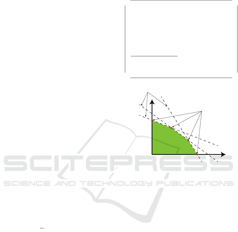
Figure 2: Existence of multiple reward functions.
3.1 Existence of Multiple Reward
Functions
In 2.3, Ng et al. showed that the reward function
leading to the optimal policy must satisfy constraint
Eq. (9). An intuitive explanation of how multiple re-
ward functions can satisfy this constraint is given in
Fig. 2. Fig. 2 show a simple example for |S | = 2.
The vertical and horizontal axes show the rewards for
states 1 and 2, respectively.
All of the reward functions in the shaded feasible
region are consistent with the optimal policy. That is,
there can be multiple reward functions satisfying con-
straint Eq. (9). In addition to satisfying the constraint,
inverse reinforcement learning can be extended to
consider the optimization of the reward function by
introducing an additional objective function. Thus,
finding the reward function that leads to the optimal
policy and finding the optimal reward function are
two separate problems. This paper deals with the lat-
ter problem.
ICAART 2018 - 10th International Conference on Agents and Artificial Intelligence
278

3.2 Related Work: Objective Function
in Reward Optimization
As described in the previous section, there are mul-
tiple reward functions that lead to the optimal policy.
Therefore when considering an actual problem, it is
necessary to unify on a single reward function. In
previous research, the determination of the objective
function is based solely on its ability to reproduce the
optimal behavior. We summarize objective functions
for inverse reinforcement learning that are representa-
tive of these studies below.
Ng et al. consider methods that determine the re-
ward function which maximizes Q value. By using
this objective function, actions other than the optimal
action in each state have a lower expected reward than
the optimal action. Therefore, those actions are less
likely to be chosen.
The optimization of Abbeel et al. (Pieter Abbeel,
2004) is
min||µ
θ
− µ
E
||, (14)
which minimizes the difference between the feature
expectation value µ
θ
learned by the estimated reward
function and the expert feature expectation value µ
E
.
The feature expectation value includes the elements
of the transition state and time, and realizes the same
behavior as the expert by selecting the weight whose
feature expectation values coincide with those of the
expert.
The objective function of Syed et al. (U. Syed and
Schapire, 2008) was proposed to improve the perfor-
mance of Abbeel ’s method, as follows:
minθ(µ
θ
− µ
E
), (15)
Since the objective function θ · µ, the product of the
weight and the feature expected value, can be re-
garded as the average expected reward, we estimate
the weight so that it becomes the average expected
reward value equivalent to that of the expert. In par-
ticular, rather than taking the difference between the
norm of the feature expectation values and using it as
the norm of the expectation reward, we make a more
accurate estimation.
Neu et al. (Neu and Szepesvari, 2007) considered
the optimization
min
∑
s∈S,a∈A
ν
E
(s)(π(a|s) − π
E
(a|s))
2
, (16)
where frequency of occurrence of each state s ∈ S is
π(a|s), and ν
E
(s) = 1/n ·
∑
N
t=s)
represents the corre-
sponding probability of taking action a. The opti-
mization directly approximates an expert’s policy.
Ziebart et al. (B. D. Ziebart and Dey, 2008) and
Babes et al. (M. Babes-Vroman and Littman, 2011)
considered the following optimization:
max
∑
ξ∈D
logP(ξ|θ), (17)
where ξ ∈ D represents one exercise action sequence,
D represents a set of action sequences, and P(ξ|θ) =
1/Z(θ)e
θµ
is the probability distribution of action se-
quence ξ given weight θ. Let P
E
(ξ) be the proba-
bility distribution of the expert’s action sequence and
P(ξ|θ) be the probability distribution of the action se-
quence for the estimated reward. Then the distribu-
tion of the KL information for the experts and esti-
mated rewards can be expressed as
∑
ξ∈D
P
E
(ξ)logP
E
(ξ)/P(ξ|θ), (18)
and so the likelihood function can be expressed as
min −
∑
ξ∈D
P
E
(ξ)
˙
logP(ξ|θ) (19)
When the amount of data is sufficient, the estimate
of the objective function converges to Eq. (17) by the
law of large numbers. Eq. (17) minimizes the differ-
ence between the probability distribution of the ex-
pert’s action sequence and the probability distribution
of the action sequence of the estimated reward. Thus,
by including this comparison between these probabil-
ity distributions, this method can be applied even if
some inaccuracies exist in the expert’s behavior se-
quence.
Although the above objective functions differ,
they estimate the reward that increase reproducibility.
3.3 Definition of Reproducibility and
Learning Efficiency
Reproducibility is not considered in previous studies,
as they do not consider the determination of a unique
objective function for the reward as shown in 3.2. In
this paper, we define reproducibility and learning ef-
ficiency as objective functions for evaluating the re-
ward function.
Reproducibility. We define the reproducibility as
the concordance rate between the optimal action a
1
of
a given policy and the action of the estimated policy
π
IRL
(s) by inverse reinforcement learning. Let f (s)
be a function over S that returns 1 when the action in
Estimation of Reward Function Maximizing Learning Efficiency in Inverse Reinforcement Learning
279

the estimated policy is the same as the action for the
given policy, and 0 otherwise:
f (s) =
1 i f max
a
π
IRL
(s) = a
1
,
0 otherwise
(20)
If M is the total number of states, then the repro-
ducibility is expressed using Eq. (20) as
1
M
∑
s∈S
f (s). (21)
Learning Efficiency. The learning efficiency is de-
fined as the sum of the number of steps for all
episodes. Here we define one step as the minimum
time required to make a decision and one episode as
the total time required to reach the target state. Specif-
ically, the learning efficiency is
N
∑
i=1
H
i
(R), (22)
where R is the the reward function, the number of
steps required for each episode i is H
i
(R), and the final
episode is N.
4 PROPOSED METHOD:
REWARD FUNCTION FOR
MAXIMIZING LEARNING
EFFICIENCY
In this section, we propose a method for estimating
the reward function for maximizing the learning effi-
ciency as defined in Section 3.3. First, we reformu-
late the inverse reinforcement learning method pro-
posed by Ng et al. to maximize the learning efficiency.
Then, we introduce a genetic algorithm (GA) in order
to solve the formulated problem efficiently.
4.1 Formulation of Inverse
Reinforcement Learning to
Maximize Learning Efficiency
The formulation of Ng et al. (Eq. (3)) consists of ob-
jective functions and constraints. The objective func-
tions increase the reproducibility and the constraints
guarantee that a given policy is feasible. Since the
purpose of this paper is to maximize learning effi-
ciency, we introduce an objective function for this.
In particular, we introduce Eq. (23) below, which has
an objective function chosen in order to minimize the
the learning efficiency given in Eq. (22) up to N
early
episodes.
min
N
early
∑
n=1
H
n
(R) (23)
Only the initial episode is used to calculate the ob-
jective function to suppress unnecessary search steps
at the early learning stage and to prevent a decrease
in the learning efficiency differences for each reward
function due to an increase in the number of episodes.
4.2 GA Approach
In solving the proposed formulation, we have two is-
sues. The first issue is that the derivative of the ob-
jective function can not be analytically determined.
The second issue is that the objective function of the
proposed method is not a convex function but a mul-
timodal function. In the gradient method which is a
well-known nonlinear optimization method is not ap-
propriate for these issues. For the first issue, since the
differential value can not be analytically obtained, nu-
merical differentiation is required and the calculation
cost becomes enormous. For the second issue, since
it is a multimodal function, the gradient method con-
verges to a local solution that depends on the initial
value with high probability.
Therefore, we introduce GA to solve these issues.
GAs are metaheuristics that do not require assump-
tions such as differentiability and multimodality of
their objective functions. Therefore, GAs can be ap-
plied to various problems due to their flexibility.
The algorithm for the proposed method is shown
as Algorithm 1. We set the l th individual of I
k
in the
kth generation population to ind
k
l
∈ I (l = 0,...,L) ,
where each individual consists of two elements: ind =
{ch, f itness}. ch = {R(s
i
)}
M
i=0
is a gene vector that
consists of the reward value of all states, and f itness ∈
R represents the adaptive degrees.
Since the GA cannot directly handle constraints,
we derive the following method to generate an indi-
vidual that satisfies the constraints. Each individual
evolves over the following two phases.
Phase 1. Search for solutions that satisfy all con-
straints
Phase 2. Search for solutions to improve the learning
efficiency
For Phase 1, we apply a penalty that is propor-
tional to the number of individuals that violated the
constraints. The individuals that satisfy all constraints
ICAART 2018 - 10th International Conference on Agents and Artificial Intelligence
280

Algorithm 1: Proposed algorithm.
1: Initialization
2: k ← 0 generation
3: for l = 0 to L do
4: for i = 0 to M do
5: ind
k
l
.ch
i
← Random(1,−1)
6: end for
7: ind
k
l
. f itness ← maxvalue
8: end for
9: Main Loop
10: for k = 1 to K do
11: for l = 1 to L do
12: Phase 1 : Satisfy constraint
13: if Eq. (9) < 0 then Violating constraints
14: ind
k
l
. f itness ← number violating con-
straints penalty
15: Phase 2 : Optimize learning efficiency
16: else if Eq. (9) > 0 then Satisfying all
constraint
17: ind
k
l
. f itness ← Eq. (23)
18: end if
19: end for
20: Genetic operation
21: Tournament Selection(I
k
)
22: Crossover(I
k
)
23: Mutation(I
k
)
24: end for
go to Phase 2, learning efficiency is calculated using
the reward function of the individual using Q learning,
and the fitness is determined according to the learning
efficiency.
An advantage of the two-phase approach is the re-
duction in the calculation time. That is, functions that
do not satisfy the constraints are reward functions that
cannot guarantee the acquisition of the optimal be-
havior. Therefore, by excluding these functions from
the search space through Phase 2, we can reduce the
computation time.
5 EXPERIMENTS
We evaluate the usefulness of the proposed method by
comparison with Ng’s and Abbeel’s methods, which
are typical inverse reinforcement learning methods.
We use the reproducibility and learning efficiency de-
fined in Section 3.3 to evaluate the performances of
the methods. The GridWorld problem is used, as it
is widely used to benchmark reinforcement learning
methods, and we vary the length of the (square) grid
from 5 to 8. This problem consists of finding the
shortest path from the start to the goal. As an exam-
ple, let Fig. 3 denote the GridWorld environment for
a 5 × 5 grid, with start coordinates (0, 0) in the lower
left corner, and the goal in the upper right corner (4,
4).
5VCTV
)QCN
Figure 3: Experimental environment.
5.1 Experiment Setting
The parameters are the range of the reward function,
−1 ≤ R ≤ 1, and the penalty coefficient λ = 0. The
genes in the GA are represented by 0’s and 1’s, and
the reward of one state is discretized into 4 bits. The
genetic operations are tournament selection, uniform
crossover, mutation, and elite selection. The num-
ber of generations for the proposed method is 10000,
the number of individuals is 100, and the parameter
value N
early
= 100 is used in Eq. (23) to calculate the
learning efficiency. The termination condition for the
Abbeel inverse reinforcement learning method is set
as τ = 0.2. We set each parameter so that the learning
efficiency is maximized.
The reproducibility and learning efficiency are
evaluated by Q learning with the reward function ob-
tained by each method from Eq. (21) and Eq. (22),
respectively. The parameters for the Q learning are
as follows: the learning rate is 0.03, the discount rate
is 0.9, and the number of episodes is 10000. The ac-
tion selection for the Q learning is ε-greedy, and ε
becomes zero after 9900 episodes.
Here, in Ng’s method, the same reward function
is obtained even if the trial is repeated due to the
use of the linear programming method. However, in
Abbeel’s method and the proposed method, different
reward functions are estimated in each trial. Abbeel’s
method estimates the feature expectation values by re-
inforcement learning, and the proposed method esti-
mates the reward function by the GA and calculates
the fitness by reinforcement learning. In these meth-
ods, randomness is inherent in the estimation of the
reward function. Therefore, to fairly evaluate the per-
formance of each algorithm, each method is applied
10 times to each environment, and 10 reward func-
tions are thus obtained. We calculate the average and
standard deviation of the reproducibility and learning
efficiency for the 100 obtained reward functions, and
use the best reward functions among the 10 reward
functions for the comparison of the methods. The to-
tal number of states M necessary to calculate the re-
producibility is the same as the number of squares in
GridWorld.
Estimation of Reward Function Maximizing Learning Efficiency in Inverse Reinforcement Learning
281
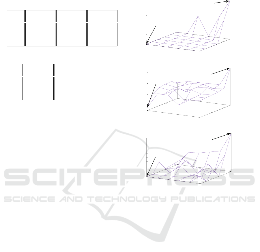
Table 1: Comparison of the reproducibility[%].
Ng Abbeel Proposed
method
5 × 5 65.4 (6.11) 62.2 (3.32) 92.3 (2.91)
6 × 6 67.0 (6.37) 51.5 (2.89) 86.3 (4.08)
7 × 7 63.3 (6.19) 51.7 (3.68) 84.4 (3.04)
8 × 8 64.9 (7.73) 56.9 (2.70) 87.3 (2.72)
Table 2: Comparison of the efficiency[10
3
].
Ng Abbeel Proposed
method
5 × 5 173(63.4) 92.7 (0.125) 91.2(0.118)
6 × 6 1470(23.6) 115 (46.3) 116 (0.147)
7 × 7 1410(94.2) 1463 (45.2) 149 (0.175)
8 × 8 295(111) 174 (0.294) 179 (0.185)
5.2 Results
The reproducibility and learning efficiency of each
method are shown in Table 1 and Table 2, respec-
tively. Bold in Table 1 and Table 2 indicates the best
results.
In terms of the reproducibility, the proposed
method performs better than the other methods (Ta-
ble 1). For the learning efficiency in the cases of the
5 × 5 and 7 × 7 grids, the proposed method again per-
forms best (see Table 2). However, Abbeel’s method
is slightly better than the proposed method for the
6 × 6 and 8 × 8 grids. The significance of the differ-
ences in the reproducibility and the learning efficiency
between the proposed method and the standard meth-
ods is compared with a t-test at the 5% significance
level. The null hypothesis states that the mean and
standard deviation of the two methods are equal to
those of the proposed method. Since the null hypoth-
esis was rejected, it is confirmed that there is a signifi-
cant difference between our proposed method and the
standard methods.
6 DISCUSSION
In this section, the reproducibilities and learning ef-
ficiencies of the existing and proposed methods are
considered based on the results of the experiments.
6.1 Evaluation of Reproducibility
From Table 1, the reproducibility of the proposed
method is about 22% and 32% higher than those of
Ng’s and Abbeel’s methods, respectively. We con-
sider the reason for this in terms of the shape of the re-
ward function for the 6×6 GridWorld of each method
0
1
2
3
4
5
0
1
2
3
4
5
-1
-0.5
0
0.5
1
X
Y
R
START
GOAL
(a) Ng
0
1
2
3
4
5
0
1
2
3
4
5
-0.4
-0.3
-0.2
-0.1
0
0.1
0.2
0.3
X
Y
R
START
GOAL
(b) Abbeel
0
1
2
3
4
5
0
1
2
3
4
5
-1
-0.8
-0.6
-0.4
-0.2
0
0.2
0.4
0.6
0.8
1
R
X
Y
START
GOAL
(c) Proposed method
Figure 4: Reward function of 6 6 GridWorld.
as shown in Fig. 4.
In the reward function obtained by the method of
Ng (Fig. 4 (a)), the reward value is given only to the
states close to the target state and the reward value is
thus 0 for most states. In states where there are two
optimal actions, it is highly likely that actions other
than the actions for which the reward is given will
be taken, so the reproducibility is low. In the reward
function obtained by Abbeel’s method (Fig. 4 (b)), the
reward value is given only to the state around the op-
timal route, so the learner takes only the optimal ac-
tions near the shortest path. In the reward function ob-
tained by the proposed method (Fig. 4 (c)), a reward
value is given for each state, so the reproducibility
is relatively high. This is the result of explicitly in-
cluding the learning efficiency in the objective func-
tion. Although the improvement in the learning effi-
ciency is introduced explicitly as the objective func-
tion, the reproducibility is reflected only in the con-
straint. However, compared with the existing meth-
ods, it was confirmed that the reproducibility is in-
creased.
ICAART 2018 - 10th International Conference on Agents and Artificial Intelligence
282

Table 3: Comparison of the efficiency of 10 trials [10
3
].
Ng Abbeel Proposed
method
5 × 5 173( 0 ) 189 (12.6) 92.0 (0.132)
6 × 6 1470 ( 0 ) 257 (86.7) 120 (0.172)
7 × 7 1410 ( 0 ) 1900 (581) 154 (0.166)
8 × 8 295 ( 0 ) 3500 (2490) 193 (0.178)
6.2 Evaluation of Learning Efficiency
From Table 2, the learning efficiency of the proposed
method was high for all GridWorld settings. The rea-
son for this is that the methods of Ng and Abbeel max-
imize only the reproducibility, whereas the proposed
method explicitly considers the learning efficiency.
On the other hand, Abbeel’s method had a slightly
higher efficiency than the proposed method in the
6×6 and 8 ×8 grids. The reason for this is that, as de-
scribed in 5.1, the same reward function is estimated
every time when repeating trials with Ng’s method,
but in Abbeel’s method and the proposed method,
there is an inherent randomness, resulting in different
estimates of the reward function with each repetition
of the trial. In other words, although Abbeel’s method
does not explicitly consider learning efficiency, a re-
ward function with a high learning efficiency can be
determined by chance over multiple trials.
In order clarify this point, the learning efficiency
and standard deviation are calculated for the ten re-
ward functions used in the experiment, and the aver-
age value and standard deviations are shown in Ta-
ble 3.
In Table 3, the standard deviation is 0 because
Ng’s method provides the same reward function for
all 10 trials. On the other hand, for Abbeel’s method,
the standard deviation is very large compared with
other methods, and thus the learning efficiency varies
widely between trials. Since the proposed method es-
timates the reward function using a GA, there is no
guarantee that it converges to the optimal solution.
Nevertheless, the standard deviation for the proposed
method is small, showing that the proposed method
can provide stable estimates for the reward function
with a high learning efficiency for each trial.
6.3 Limits of the Proposed Method
In GridWorld environments larger than 8×8, the pro-
posed method could not obtain a solution that satisfies
all of the restrictions presented in Eq. (9). It is rea-
sonable to suppose that since the executable area is
narrowed by increasing the number of constraints and
states, it is difficult to search the executable area with
a simple penalty method. In particular, a drawback
of the GA method is that it cannot explicitly handle
constraints.
7 CONCLUSION
In this paper, we proposed an inverse reinforcement
learning method for finding the reward function that
maximizes the learning efficiency. In our proposed
method, an objective function for the learning effi-
ciency is introduced using the framework of the in-
verse reinforcement learning of Ng et al. Moreover,
since our proposed objective function is nonlinear and
convex, we find the solution using a GA.
A limitation of the method proposed in this paper
is that the GA cannot always converge to an optimal
solution when the number of states is too high, so fu-
ture work will consider the following: 1) relaxation of
the constraints, 2) formulation of our method as a lin-
ear or quadratic programming problem, and 3) appli-
cation of a strong GA for finding solutions satisfying
the constraints.
REFERENCES
Andrew Y. Ng, Daishi Harada, S. R. (1999). Policy invari-
ance under reward transformations: Theory and appli-
cation to reward shaping. In International Conference
on Machine Learning.
B. D. Ziebart, A. Maas, J. A. B. and Dey, A. K. (2008).
Maximum entropy inverse reinforcement learning. In
The AAAI Conference on Artificial Intelligence.
M. Babes-Vroman, V. Marivate, K. S. and Littman, M.
(2011). Apprenticeship learning about multiple inten-
tions. In International Conference on Machine Learn-
ing.
Neu, G. and Szepesvari, C. (2007). Apprenticeship learn-
ing using inverse reinforcement learning and gradient
methods. In annual Conference on Uncertainty in Ar-
tificial Intelligence.
Ng, A. Y. and Russell, S. (2000). Algorithms for inverse
reinforcement learning. In International Conference
on Machine Learning.
Pieter Abbeel, A. Y. N. (2004). Apprenticeship learning
via inverse reinforcement learning. In International
Conference on Machine Learning.
Richard S. Sutton, A. G. B. (2000). Reinforcement Learn-
ing: An Introduction. Xko.
U. Syed, M. B. and Schapire, R. E. (2008). Apprenticeship
learning using linear programming. In International
Conference on Machine Learning.
Estimation of Reward Function Maximizing Learning Efficiency in Inverse Reinforcement Learning
283
