
Automatic Counting and Classification of Microplastic Particles
Javier Lorenzo-Navarro
1
, Modesto Castrill
´
on-Santana
1
, May G
´
omez
2
, Alicia Herrera
2
and Pedro A. Mar
´
ın-Reyes
1
1
Instituto Universitario Sistemas Inteligentes y Aplicaciones Num
´
ericas en Ingenier
´
ıa (SIANI),
Universidad de Las Palmas de Gran Canaria, Las Palmas de Gran Canaria, Spain
2
Marine Ecophysiology Group (EOMAR), Instituto Universitario ECOAQUA,
Universidad de Las Palmas de Gran Canaria, Las Palmas de Gran Canaria, Spain
Keywords:
Microplastics, Beach Pollution, Automatic Counting, Microplastics Classification.
Abstract:
Microplastic particles have become an important ecological problem due to the huge amount of plastics debris
that ends up in the sea. An additional impact is the ingestion of microplastics by marine species, and thus
microplastics enter into the food chain with unpredictable effects on humans. In addition to the exploration of
their presence in fishes, researchers are studying the presence of microplastics in coastal areas. The workload
is therefore time consuming, due to the need to carry out regular campaigns to quantify their presence in the
samples. So, in this work a method for automatic counting and classifying microplastic particles is presented.
To the best of our knowledge, this is the first proposal to address this challenging problem. The method makes
use of Computer Vision techniques for analyzing the acquired images of the samples; and Machine Learning
techniques to develop accurate classifiers of the different types of microplastic particles that are considered.
The obtained results show that making use of color based and shape based features along with a Random
Forest classifier, an accuracy of 96.6% is achieved recognizing four types of particles: pellets, fragments, tar
and line.
1 INTRODUCTION
The use of plastics is very widespread in our society
due to the properties that make them superior to other
materials in many applications. The worldwide pro-
duction of plastics without including PET-, PA-, PP-
and polyacryl-fibers was 322 million tonnes in 2015
(Plastic Europe, 2016). Among those properties, the
plastics in general have good resistance to corrosion
and chemicals, low costs and good durability. How-
ever, those properties make the plastics one of the
most difficult debris to treat; and a part of this debris
ends up in the sea, producing an ecological problem
(Galgani et al., 2013). An estimation due to Jambeck
et al. (Jambeck et al., 2015) establishes that over 8
million tonnes of plastic enter the marine environment
annually.
The plastics in the sea can be categorized accord-
ing to their size. One category is the ”microplas-
tics” which correspond to small microplastic parti-
cles (Thompson et al., 2004; Arthur et al., 2009).
Microplastics can also be subdivided into two sub-
categories: primary microplastics which are those
that are produced as micron-sized particles; and sec-
ondary microplastics that correspond to fragments of
the breakdown of larger plastics debris (Besley et al.,
2017). As it was stated before, the good durability of
plastics results in an accumulation in the marine envi-
ronment of the microplastics that due to their reduced
size can be ingested by a wide variety of organisms
(Set
¨
al
¨
a et al., 2014).
An indirect measure of the amount of microplas-
tics in the sea is measuring the number and type
of particles that arrive to the beaches, that is also a
source of beach pollution by itself. This topic has
received a growing attention in the biology literature
(Van Cauwenberghe et al., 2015). In order to com-
pare results from different studies, it is necessary to
define a common protocol in sampling, extraction and
quantification of the microplastics particles (Shim and
Thomposon, 2015). It is in the quantification task
where this work proposes an automatic approach that
not only counts the number of microplastics particles,
but it also classifies into different categories. After re-
vieweing the literature, to the best of our knowledge,
this paper proposes the first attempt to automatically
address this challenging problem.
Due to the recent interest that has received the
646
Lorenzo-Navarro, J., Castrillón-Santana, M., Gómez, M., Herrera, A. and Marín-Reyes, P.
Automatic Counting and Classification of Microplastic Particles.
DOI: 10.5220/0006725006460652
In Proceedings of the 7th International Conference on Pattern Recognition Applications and Methods (ICPRAM 2018), pages 646-652
ISBN: 978-989-758-276-9
Copyright © 2018 by SCITEPRESS – Science and Technology Publications, Lda. All rights reserved
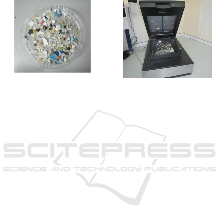
Figure 1: Sample of microplastics obtained in a beach of
Canary Islands.
study of microplastics in the sand, and the lack of a
standardized protocol in the quantification of the par-
ticles, we are not aware of any automatic approach to
solve this task. Currently, researchers count and iden-
tify manually the particles that appears in a sample
(Figure 1) that is a very time consuming process. In
some cases, the use of image processing software can
be used to alleviate this task, but in the end the re-
searchers have to classify the particles using the met-
rics obtained with the image processing tool.
A similar task to the microplastics analysis is the
study of the zooplankton which is also very time con-
suming because it requires to count and classify the
different species that appear in a sample; in the same
way that must be done with microplastics samples.
In the zooplankton analysis, ZooImage tool (Gros-
jean and Denis, 2014) has been used to the automated
classification of zooplankton species (Irigoien et al.,
2008; Bachiller et al., 2012; Medellin-Mora and Es-
cribano, 2013). ZooImage is an opensource solution
written in R and that makes use of ImageJ image
analysis tool to obtain different statistics of the zoo-
plankton samples as abundances, total and partial size
spectra or biomasses, etc. The accuracy of the first
version of ZooImage was evaluated in (L. Bell and
R. Hopcroft, 2008), reporting an accuracy over 70%,
but it varies depending of the species and the size of
them. Similar evaluations have not been reported for
recent versions of the software. ZOOSCAN (Gros-
jean et al., 2004) is another software that allows the
automatic counting of zooplankton samples and the
semi-automatic identification of taxa with accuracy
rates about 75% similar to ZooImage.
Some researchers have applied ZooImage to mi-
croplastics with poor results due to the fact that this
tool compute a set of features mainly based on optical
density. Those features are well suited for identifying
zooplankton species but they are not the best ones for
Figure 2: Sample of microplastics obtained in a beach of
Canary Islands.
microplastic particles that are mainly opaque. Thus,
researchers must do the work manually, while de-
manding a simple and adopted solution for this prob-
lem.
In this paper, an approach for counting and clas-
sifying microplastic particles is presented integrat-
ing both Computer Vision as Machine Learning tech-
niques. The main contributions of the paper can be
summarized as: 1) automatic counting detection of
microplastic particles in a sample image, and 2) auto-
matic classification of the particles into four types of
interest.
2 METHODOLOGY
In recent years, the use of the Deep Learning ap-
proaches for object classification (Krizhevsky et al.,
2012; Simonyan and Zisserman, 2014; Girshick,
2015; Szegedy et al., 2015) have exhibited a perfor-
mance in complex tasks like never before. Obviously,
the problem of microplastics classification could be
solved with a Deep Learning approach but the lack of
thousands of labeled samples hinders the training pro-
cess. Thus, the proposed approach follows the clas-
sical pattern recognition pipeline (Duda et al., 2001)
with the following stages: image acquisition, image
segmentation, feature extraction and classification.
2.1 Image Acquisition
Images acquisition is performed using a high defini-
tion scanner due to the small size of the microplas-
tic particles (0.3-5 mm) after distributing the particles
over the scanning platform (Figure 2). This is done
similarly to the requirements imposed by ZooImage.
These images have a high resolution that goes from
Automatic Counting and Classification of Microplastic Particles
647
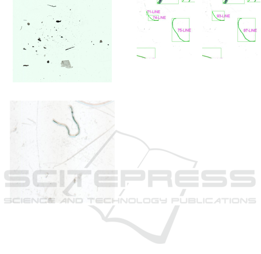
Figure 3: Crop of an image of a microplastics sample.
Figure 4: Background detail with creases and a line mi-
croplastic particle.
aproximately 4800x6900 pixels to 9700x13800 pixels
depending on the scanner configuration. These high
resolution images avoid the loss of details in the par-
ticles but it has the drawback that reveals any imper-
fection of the background. Figure 4 shows this effect
where some creases can be mixed up with the line that
appear in the image. This fact introduced a source of
noise in the identification of some types of microplas-
tics, specifically the lines.
2.2 Image Segmentation
Due to the nature of the images that are obtained by
means of a scanner, the background is clear and the
particles are normally darker as can be seen in Figure
3. The first task is to obtain the connected components
(blobs) that are candidate to be microplastic particles.
This task can be carried out by means of a threshold-
ing technique where pixels with a value higher than
a threshold are considered background. In the liter-
ature, there are a bunch of thresholding algorithms
Figure 5: Fishing line
segmentation using Otsu’s
method.
Figure 6: Fishing line seg-
mentation using Sauvola’s
method.
(Sezgin and Sankur, 2004). They can be grouped
into global methods when a single threshold value is
used in the whole image; and adaptive methods when
the threshold value is calculated at each pixel, which
depends on some local statistics. Among the global
methods, one of the most widely used is the Otsu’s
method (Otsu, 1979) that gives good results when the
regions are not linear. In the problem of microplastic
particles, one type is due to the breakdown of fish-
ing lines or nets and their shape is very linear. For
this kind of particles, Otsu’s method does not pro-
duce good results because it is prone to divide lin-
ear blobs into several parts. To avoid this drawback
the adaptive threshold method proposed by Sauvola
and Pietik
¨
ainen (Sauvola and Pietik
¨
ainen, 2000) has
been used. A comparison between the results of both
methods applied to a fishing line particle are shown
in Figures 5 and 6. It is observed that the particle
93-LINE of Figure 6, in Figure 5 appears as two par-
ticles, 71-LINE and 74-LINE.
2.3 Feature Extraction
The features obtained for each blob can be grouped
into two categories: color and geometric features.
Into the first category, the features are computed over
each blob pixel and those are:
• Average and variance of the gray level of the blob
pixels.
• Average and variance of the RGB components of
the blob pixels.
• Average and variance of the HSV components of
the blob pixels.
The second category of features includes all those
features that are related with the shape of the blob.
Those features are:
• Compactness of the blob computed as
perimeter
2
/area.
• Ratio between the area of the blob and its bound-
ing box.
ICPRAM 2018 - 7th International Conference on Pattern Recognition Applications and Methods
648
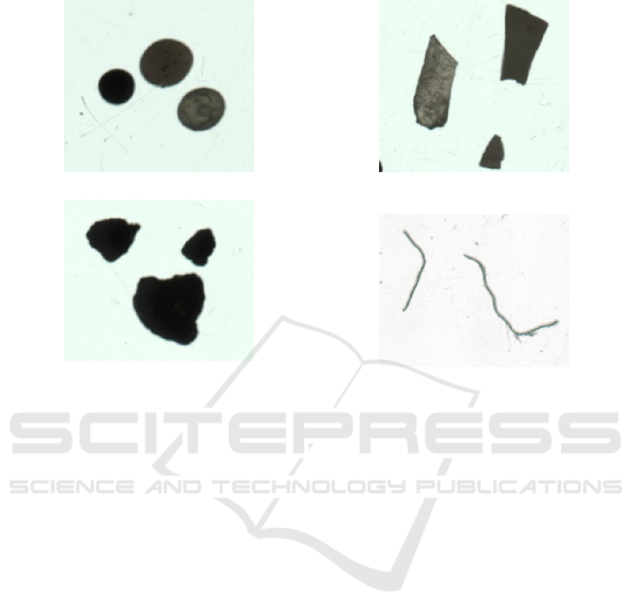
a) Pellet. b) Fragment.
c) Tar.
d) Line.
Figure 7: Details of microplastics and tar particles captures.
• Ratio between the width and the height of the blob
bounding box.
• Ratio between the major and minor axis of the fit-
ted ellipse.
• Ratio between the major and minor radius defined
as the distance from the furthest and closest pixel
of the contour to the centroid of the blob.
2.4 Classification
As it was stated before, the lack of a huge amount of
labeled images makes difficult to train a deep learn-
ing based approach as a Convolutional Neural Net-
work (Lecun et al., 1998). For this reason, some well
known Machine Learning supervised methods are go-
ing to be used, specifically K Nearest-Neighbor, C4.5,
Random Forest, Adaptive Boosting and Support Vec-
tor Machine. In the following paragraphs, a brief de-
scription of each method is given.
K Nearest-Neighbor (K-NN). This method belongs
to the case-based classifiers (Aha et al., 1991)
which store all the training instances. Later, the
classification of a new sample is performed con-
sidering the K nearest training samples to it. The
class assigned to the test sample is given using a
voting strategy among the K nearest training sam-
ples. Different values of K, distances measures
to get the nearest neighbors and voting strategies
have been proposed in the literature.
C4.5. This classifier is a decision tree (Quinlan,
1993) which is built in a top-down manner. Train-
ing samples are divided in each node according to
the best attribute of the subset of training samples
that correspond to the node. The stopping crite-
ria is when all samples that correspond to a node
belong to the same class or the best split of the
node does not surpass a fixed Chi-square signifi-
cant threshold. After the growing stage, a pruning
phase is realized to avoid overfitting.
Random Forest (RF). This classifier is made up of
several decision trees which are built using sub-
sets of the training samples randomly selected
with replacement (Breiman, 2001). In the grow-
ing stage of each tree, in each node a set of ran-
domly attributes is considered obtaining in this
way uncorrelated trees. To classify a new sam-
ple, after feeding it into all the trees, a majority
strategy is used to assign the class to the sample.
Support Vector Machine (SVM). This classifier ob-
tains the hyperplanes that separate the training
samples of different classes minimizing the ex-
pected error (Vapnik, 1999). The support vec-
tor are those samples that define the hyperplanes.
For non linear separables classes, the original
Automatic Counting and Classification of Microplastic Particles
649
space is transformed using kernels where the most
frequently used are polynomial and radial based
(RBF).
Adaptive Boosting (AdaBoost). Boosting is an ap-
proach in Machine Learning that builds high ac-
curate classifiers based on weak ones. Adaptive
Boosting (Freund, 2001) is one of the most widely
used boosting algorithms. In AdaBoost algo-
rithms, the weak classifiers are iteratively trained
using the misclassified samples of the previous
classifier, in this way, each classifier refines the
outcome of the previous one.
3 EXPERIMENTS AND RESULTS
In this work, four categories of microplastics are con-
sidered (see Figure 7). A brief description of them is
given below.
Pellet. This category corresponds to small beads of
primary microplastics.
Fragment. This category corresponds to small frag-
ments derived from the breakdown of larger plas-
tic debris.
Line. This category corresponds to small part of fish
lines or nets.
Tar. Although it is not a plastic polymer, this cat-
egory is included because it represents an im-
portant fraction of marine debris in coastal areas
(Herrera et al., 2017). These tar wastes are likely
to come from ships that discharge bunker oil at
sea, or from old oil spills deposited on rocks and
fragmented by action of waves, producing small
solid tar fragments.
For the experimental setup, the particles are ob-
tained from four images containing a total of 844 in-
stances: 342 pellet particles, 227 fragment particles,
174 tar particles and 101 line particles. For each par-
ticle, the 19 features described in section 2.3 are com-
puted, and the five classifiers are trained using a 10-
fold cross validation setup.
For the AdaBoost classifier, a simple linear regres-
sion logistic was used as weak classifier. The number
of neighbors in the K-NN classifier was set to 1 (K=1)
via cross validation and euclidean distance as distance
function. The SVM classifier was trained with RBF
kernel and with parameter C=12 whose value was
tuned by cross-validation.
The accuracy obtained for each classifier is shown
in Table 1. According to the results, the classifier with
the lowest performance is the SVM with 91.1 of ac-
curacy. AdaBoost, K-NN and C4.5 give similar ac-
curacy around 93 and the classifier with the highest
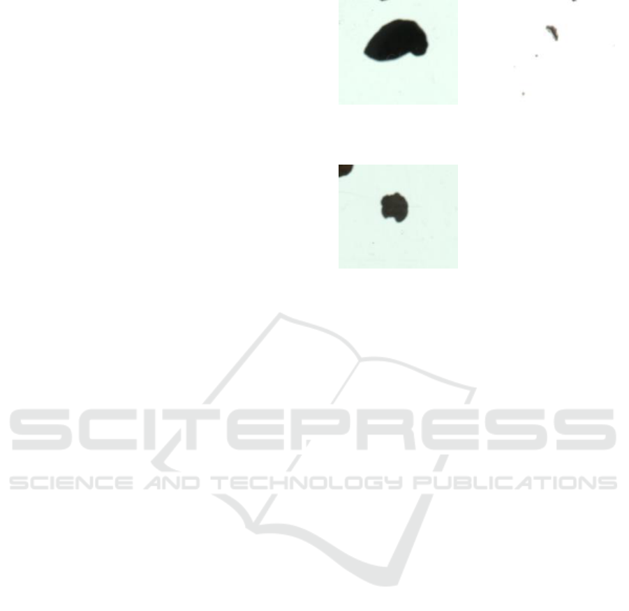
a) Fragment classified as
tar.
b) Line classified as tar.
c) Pellet classified as frag-
ment.
Figure 8: Examples of classification errors.
accuracy is the Random Forest that yields 96.6. In
Table 1, it can be also observed that for all the clas-
sifiers, the values of recall and precision are close to
the accuracy which implies a similar performance of
the classifiers for the four classes.
In order to assess if there exists redundancy
among the computed features, a feature selection and
feature projection processes prior to train the Ran-
dom Forest were carried out. For feature selection
we adopted the ReliefF method (Kononenko, 1994)
which tries to find those features that maximize the
separation of the classes. The best result was obtained
using 17 features, two less than the original feature
set, with an accuracy of 96.6. Those removed were
Ratio between the width and the height of the blob
bounding box and Ratio between the major and minor
axis of the fitted ellipse. The projection of the feature
set was done with the Principal Component Analysis
keeping the 95 of the initial variability, resulting in a
7-dimension space. The accuracy of the Random For-
est using the projected features was 95.5.
The confusion matrix for the Randon Forest with
the selected features is shown in Figure 9. Though
the Random Forest in general does not produce too
much missclassification, it can be observed that the
most are with the fragment category. This is due to the
high variability in shape and color of this kind of mi-
croplastics because they come from large plastic de-
bris. In Figure 8, some missclassifications are shown.
In most cases, these misclassification errors are dif-
ficult to overcome even for experts. In this sense,
texture descriptors may introduce additional informa-
tion. The computation of these descriptors was done
ICPRAM 2018 - 7th International Conference on Pattern Recognition Applications and Methods
650
Table 1: Results of microplastics classification (%)
Classifier Accuracy Precision Recall
AdaBoost 93.5 93.5 93.5
K-NN (K=1) 93.7 93.9 93.7
C4.5 92.4 92.4 92.4
Random Forest 96.4 96.5 96.4
SVM (C=12) 91.1 91.1 91.1
ReliefF + Random Forest 96.6 96.6 96.6
PCA + Random Forest 95.5 95.6 95.5
using the same blobs that those used for computing
the color features. As a prospective test, the Weber
Local Descriptor (Chen et al., 2010) was computed
for the classes Fragment, Pellet and Tar; and a Ran-
dom Forest was trained in a 10 cross-validation setup
obtaining an accuracy of 88.5%. If this kind of texture
descriptors are combined with those presented in this
paper, we expect that the overall performance could
improve.
Figure 9: Confusion matrix for the Random Forest.
Classified as
Pellet Fragment Tar Line
Pellet 338 4 0 0
Fragment 10 206 10 0
Tar 0 3 171 0
Line 0 1 0 100
4 CONCLUSIONS
In this paper, a method for counting and classi-
fying microplastic particles has been presented ex-
hibiting promising results. The method makes use
of both Computer Vision techniques and Machine
Learning algorithms. The use of a adaptive thresh-
olding method that takes into account the linear shape
of one type of microplastic particle has improved the
segmentation results.
Five different classification methods were tested
to assess their performance in classifying the four
types of microplastics considered in this work. To
train and test the classifiers, 14 color-based and 5
shape-based features were computed on each detected
particle. This feature set has proved to have enough
discrimination ability to differentiate among the mi-
croplastics under consideration because for all the
classifiers the accuracy was higher than 90%. The
best result was obtained with the Random Forest clas-
sifier, using the 17 most informative features, that
yields an accuracy of 96.6%.
After this preliminary results, even when there is
no study about the acceptable error measuring the
presence of microplastics, experts seem to be more
interested in having an automatic tool that saves lots
of time, even if classification errors would be around
10%. As already mentioned, manual counting is a
time consuming task affected seriously by fatigue,
therefore not free of errors even if done by human
experts. However, in order to increase this accuracy,
a transfer learning approach can be used with pre-
trained convolutional network and doing a fine tuning
with the microplastics labeled samples.
ACKNOWLEDGEMENTS
This work has been partially funded by the Departa-
mento de Inform
´
atica y Sistemas of the Universidad
de Las Palmas de Gran Canaria.
REFERENCES
Aha, D. W., Kibler, D., and Albert, M. K. (1991). Instance-
based learning algorithms. Machine Learning, 6:37–
66.
Arthur, C., Baker, J., and Bamford, H., editors (2009). Pro-
ceedings of the International Research Workshop on
the Occurrence, Effects and Fate of Microplastic Ma-
rine Debris, number NOS-OR&R-30 in NOAA Tech-
nical Memorandum.
Bachiller, E., Fernandes, J., and Irigoien, X. (2012). Im-
proving semiautomated zooplankton classification us-
ing an internal control and different imaging devices.
Limnology and oceanography, methods, 10:1–9.
Besley, A., Vijver, M. G., Behrens, P., and Bosker, T.
(2017). A standardized method for sampling and
extraction methods for quantifying microplastics in
beach sand. Marine Pollution Bulletin, 114(1):77 –
83.
Breiman, L. (2001). Random forests. Machine Learning,
45(1):5–32.
Chen, J., Shan, S., He, C., Zhao, G., Pietik
¨
ainen, M., Chen,
X., Gao, W. (2010). WLD: A Robust Local Image
Descriptor. IEEE Transactions on Pattern Analysis
and Machine Intelligence,32(9), 1705–1720.
Duda, R. O., Hart, P. E., and Stork, D. G. (2001). Pattern
Classification (2nd Edition). Wiley-Interscience.
Automatic Counting and Classification of Microplastic Particles
651

Freund, Y. (2001). An adaptive version of the boost by ma-
jority algorithm. Machine Learning, 43(3):293–318.
Galgani, F., Hanke, G., Werner, S., and De Vrees, L.
(2013). Marine litter within the european marine strat-
egy framework directive. ICES Journal of Marine Sci-
ence, 70(6):1055–1064.
Girshick, R. (2015). Fast r-cnn. In Proceedings of the 2015
IEEE International Conference on Computer Vision
(ICCV), ICCV ’15, pages 1440–1448, Washington,
DC, USA. IEEE Computer Society.
Grosjean, P. and Denis, K. (2014). zooimage: Analysis of
numerical zooplankton images.
Grosjean, P., Picheral, M., Warembourg, C., and Gorsky,
G. (2004). Enumeration, measurement, and identifi-
cation of net zooplankton samples using the zooscan
digital imaging system. ICES Journal of Marine Sci-
ence, 61(4):518–525.
Herrera, A., Asensio, M., Mart
´
ınez, I., Santana, A.,
Packard, T., and G
´
omez, M. (2017). Microplastic and
tar pollution on three canary islands beaches: An an-
nual study. Marine Pollution Bulletin. In press.
Irigoien, X., Fernandes, J., Grosjean, P., Denis, K., Albaina,
A., and Santos, M. (2008). Spring zooplankton distri-
bution in the bay of biscay from 1998 to 2006 in re-
lation with anchovy recruitment. Journal of Plankton
Research, 31.
Jambeck, J. R., Geyer, R., Wilcox, C., Siegler, T. R., Per-
ryman, M., Andrady, A., Narayan, R., and Law, K. L.
(2015). Plastic waste inputs from land into the ocean.
Science, 347(6223):768–771.
Kononenko, I. (1994). Estimating attributes: Analysis and
extensions of RELIEF. In Bergadano, F. and de Raedt,
L., editors, Machine Learning: ECML-94, pages 171–
182, Berlin. Springer.
Krizhevsky, A., Sutskever, I., and Hinton, G. E. (2012). Im-
agenet classification with deep convolutional neural
networks. In Proceedings of the 25th International
Conference on Neural Information Processing Sys-
tems - Volume 1, NIPS’12, pages 1097–1105, USA.
Curran Associates Inc.
L. Bell, J. and R. Hopcroft, R. (2008). Assessment of
zooimage as a tool for the classification of zooplank-
ton. Journal of Plankton Research, 30.
Lecun, Y., Bottou, L., Bengio, Y., and Haffner, P. (1998).
Gradient-based learning applied to document recogni-
tion. In Proceedings of the IEEE, volume 86, pages
2278 – 2324.
Medellin-Mora, J. and Escribano, R. (2013). Automatic
analysis of zooplankton using digitized images: State
of the art and perspectives for latin america. Latin
American Journal of Aquatic Research, 41:29–41.
Otsu, N. (1979). A Threshold Selection Method from Gray-
level Histograms. IEEE Transactions on Systems,
Man and Cybernetics, 9(1):62–66.
Plastic Europe (2016). Plastics - the facts 2016.
Quinlan, J. R. (1993). C4.5: Programs for Machine Learn-
ing. Morgan Kauffman Pub., Inc., Los Altos, Califor-
nia.
Sauvola, J. and Pietik
¨
ainen, M. (2000). Adaptive document
image binarization. Pattern Recognition, 33:225–236.
Set
¨
al
¨
a, O., Fleming-Lehtinen, V., and Lehtiniemi, M.
(2014). Ingestion and transfer of microplastics in
the planktonic food web. Environmental Pollution,
185(Supplement C):77 – 83.
Sezgin, M. and Sankur, B. (2004). Survey over image
thresholding techniques and quantitative performance
evaluation. Journal of Electronic Imaging, 13(1):146–
168.
Shim, W. J. and Thomposon, R. C. (2015). Microplastics in
the ocean. Archives of Environmental Contamination
and Toxicology, 69(3):265–268.
Simonyan, K. and Zisserman, A. (2014). Very deep con-
volutional networks for large-scale image recognition.
CoRR, abs/1409.1556.
Szegedy, C., Liu, W., Jia, Y., Sermanet, P., Reed, S. E.,
Anguelov, D., Erhan, D., Vanhoucke, V., and Rabi-
novich, A. (2015). Going deeper with convolutions.
In CVPR, pages 1–9. IEEE Computer Society.
Thompson, R. C., Olsen, Y., Mitchell, R. P., Davis, A.,
Rowland, S. J., John, A. W. G., McGonigle, D., and
Russell, A. E. (2004). Lost at sea: Where is all the
plastic? Science, 304(5672):838–838.
Van Cauwenberghe, L., Devriese, L., Galgani, F., Robbens,
J., and Janssen, C. R. (2015). Microplastics in sed-
iments: A review of techniques, occurrence and ef-
fects. Marine Environmental Research, 111(Supple-
ment C):5 – 17. Particles in the Oceans: Implication
for a safe marine environment.
Vapnik, V. (1999). The Nature of Statistical Learning The-
ory. Springer-Verlag.
ICPRAM 2018 - 7th International Conference on Pattern Recognition Applications and Methods
652
