
CNN based Mitotic HEp-2 Cell Image Detection
Krati Gupta, Arnav Bhavsar and Anil K. Sao
School of Computing & Electrical Engineering, Indian Institute of Technology Mandi, Mandi (HP), India
Keywords:
Mitotic Cells, HEp-2 cells, Auto-immune Disorders, Computer-Aided Detection (CAD), CNN Architecture,
Support Vector Machines, AlexNet Architecture.
Abstract:
We propose a Convolutional Neural Network (CNN) framework to detect the individual mitotic HEp-2 cells
against non-mitotic cells, which is important for Computer-Aided Detection (CAD) system for auto-immune
disease diagnosis. The significant aspect of detecting mitotic HEp-2 cells is to consider the distinctive appear-
ance differences between the mitotic and non-mitotic classes that are represented through the learned features
from pre-trained CNN. We especially focus on gauging the effectiveness of learned features from different
CNN layers, combined with traditional Support Vector Machine (SVM) classifier. We also consider the class
sample skew between the classes. Importantly, we compare and discuss the performance of learned feature
representations, and show that some of these features are indeed very effective in discriminating mitotic and
non-mitotic cells. We demonstrate a high classification performance using the proposed framework.
1 INTRODUCTION
Indirect ImmunoFluorescence (IIF) imaging is con-
sidered to be a ‘gold standard’ to characterize the
presence of Anti-Nuclear Antibody (ANA), in order
to diagnose a connective tissue disorder i.e. autoim-
mune disorders (Kumar Y, 2009; Foggia et al., 2013;
Hobson et al., 2016). Here HEp-2 cells are used as
substrate, in which different antibodies on cells are
visualized in form of distinct nuclear staining pat-
terns in images and can be utilized to develop an ef-
ficient CAD system for aiding diagnosis. The promi-
nent nuclear staining patterns show some significance
in detection of staining patterns-specific antigens and
the associated diseases. Due to subjective & semi-
quantitative procedure, manual handling errors, intra-
personnel and laboratory variations (Foggia et al.,
2013; Hobson et al., 2014), the manual protocol of
detection requires to be aided with a CAD system
that can efficiently identify and detect the presence of
staining patterns and associated diseases, in order to
aid pathologists for obvious and non-ambiguous cases
and reduce their work pressure.
The staining patterns generated on HEp-2 is based
on the bonding between auto-antibodies to the cell
components at different stages of the cell cycle. The
staining patterns in a cell are visualized mainly in two
cell cycle stages: interphase and mitosis stages (Tonti
et al., 2015). As yet, most automated approaches have
explored the classification schemes on dominant pat-
terns of interphase stage (Hobson et al., 2016; Gupta
et al., 2016; Gupta et al., 2014; Manivannan et al.,
2016). However, the detection of mitotic type cells is
also an important and principal step in HEp-2 screen-
ing framework (Miros et al., 2015) as the antigens
released by the mitotic cells and their concentration
are responsible for some lethal diseases. Also the
identification of mitotic pattern cells is a beneficial
indication for narrowing down the patient cell pat-
terns. According to the literature, it is noticed that the
mitotic cell detection problem can be addressed us-
ing the secondary counter-stain during staining pro-
cedure, which is not an economical process. Thus,
in the present work, we primarily focus on the prob-
lem of mitotic cell detection, using only the primary
counter-stain, which is itself a novel problem defi-
nition. Moreover, due to rare occurrence of mitotic
samples, the sample imbalance between the mitotic
and non-mitotic class during classification is also an
important concern in this case. Therefore, for a com-
plete screening system, it is crucial to consider mitotic
phase cells also.
To the best of our knowledge, few authors have an-
alyzed such mitotic cell detection problem for HEp-2
cases. For instance, in (Iannello et al., 2014; Fog-
gia et al., 2010), authors have proposed a mitotic v/s
interphase/non-mitotic cell classification criteria on
a very less number of samples using morphological
Gupta, K., Bhavsar, A. and Sao, A.
CNN based Mitotic HEp-2 Cell Image Detection.
DOI: 10.5220/0006721501670174
In Proceedings of the 11th International Joint Conference on Biomedical Engineering Systems and Technologies (BIOSTEC 2018) - Volume 2: BIOIMAGING, pages 167-174
ISBN: 978-989-758-278-3
Copyright © 2018 by SCITEPRESS – Science and Technology Publications, Lda. All rights reserved
167
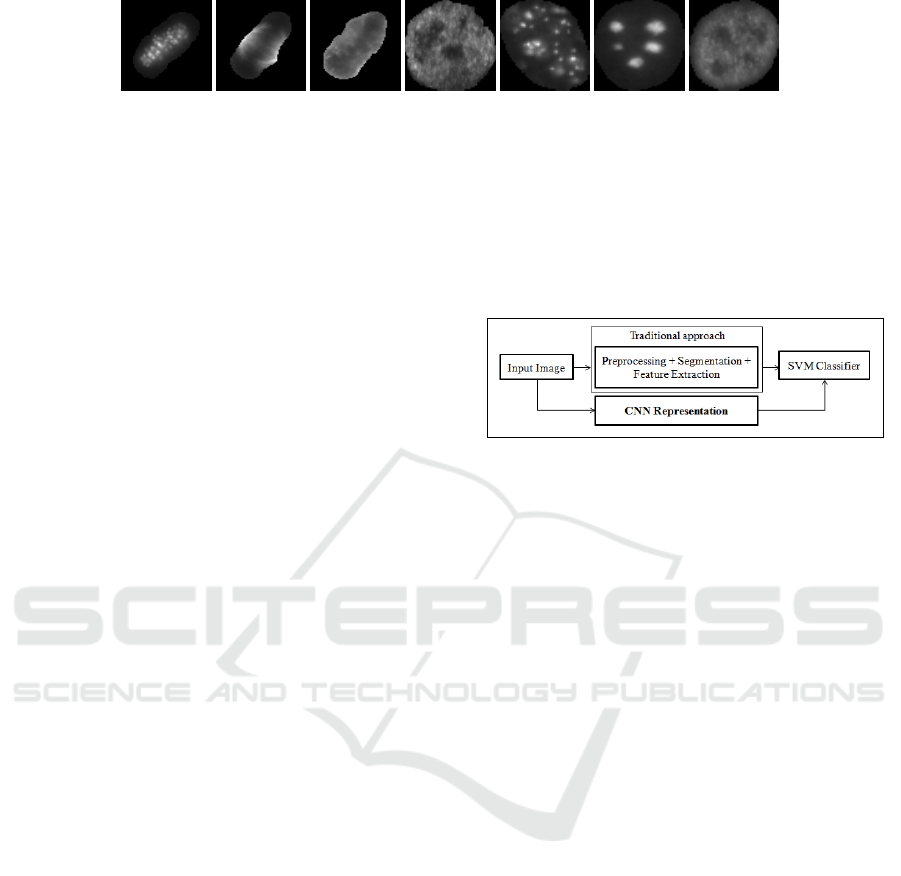
(a) (b) (c) (d) (e) (f) (g)
Figure 1: Some examples of cell images (a) to (c) mitotic cells & (d) to (g) non-mitotic cells.
and textural feature representation. In (Percannella
et al., 2011), the authors have addressed the chal-
lenge of class sample skew or imbalance and have
reviewed methods to handle the same. However,
these approaches do not consider any standard pub-
licly available dataset. In this work, we evaluate our
approach using publicly available standard dataset,
which would set a benchmark and help in compara-
tive analysis of future studies.
In the proposed work, we focus on the classifica-
tion of mitotic v/s non-mitotic cell images using fea-
tures learned by a CNN. In current scenario of pattern
recognition based works, CNNs have been proved to
be efficient and reliable models to achieve remark-
able performance for image classification and object
detection tasks. Moreover, pre-trained CNN archi-
tectures can also perform an important role in terms
of feature extractors. Hence, as a part of the work,
we also analyze the effectiveness of features learned
from different layers of the CNN. As we focus on con-
sidering the effectiveness of the features (and not on
using a complex non-linear classification model), we
use the features in a standard linear SVM, which is
a popular linear classifier. In current work, we ex-
tract features from the layers of a pre-trained AlexNet
architecture (Krizhevsky et al., 2012). The main con-
tributions of the work are as follows:
(I) Generally, a visual clear distinction can be ob-
served between the mitotic and non-mitotic classes.
Such distinction can be seen in few examples of mi-
totic and non-mitotic cells, shown in Figure 1. Fig-
ures 1(a) to 1(c) are mitotic cells, while the remaining
cells are non-mitotic. Considering this, we demon-
strate that the learned feature representation through
CNN layers can be effective in capturing such a dis-
tinction between the two types of cells, even when
using the features from a CNN which is pre-trained
on scene/object images. In this work, for the feature
extraction task, we use the pre-trained AlexNet archi-
tecture.
(II) We also focus on an important aspect of the
problem, i.e. class sample skew between the mitotic
v/s non-mitotic classes, wherein the mitotic (i.e. the
positive class) samples are very less in number, than
non-mitotic ones. Hence, we apply two standard data
skew handling strategies: undersampling and over-
sampling, and draw some useful insights.
(III) In addition to classification, we experimen-
tally analyze the effectiveness of features learned at
different CNN layers (low-level, mid-level and high-
level features), and also provide a (standard) low-
dimensional visual representation to support the ex-
perimental results.
Figure 2: Block diagram of the traditional approach v/s
CNN based classification approach.
(IV) In Figure 2, we have shown the block di-
agram of both a conventional and a CNN based
classification approach. Traditional classification
approaches typically involve steps such as pre-
processing, segmentation and feature extraction task.
Distortions in any of these tasks can accumulate and
lead to inaccuracies. The proposed application of
CNN is independent of pre-processing and segmen-
tation. Here, the entire cell image is treated as in-
put, while in case of traditional feature extraction ap-
proaches, the feature representation task is highly de-
pendent on the selection of an appropriate Region-
of-Interest (ROI) (e.g. (Iannello et al., 2014; Foggia
et al., 2010)). Hence, such a work also demonstrates
the usefulness of segmentation-free classification for
cell images.
2 PROPOSED APPROACH
As mentioned earlier, we use the learned feature rep-
resentation from CNN architecture for classification
of mitotic v/s non-mitotic class samples and analyz-
ing the effect of feature representation extracted from
different layers of CNN. More specifically, the fea-
ture responses used in this work are from the conv1,
conv2, conv3, conv4, conv5, and pool5 layers of a
pre-trained AlexNet architecture. Thus we extract
the feature representation of individual images from
a CNN and then apply the same features in SVM,
in order to get the better discrimination between the
classes.
BIOIMAGING 2018 - 5th International Conference on Bioimaging
168
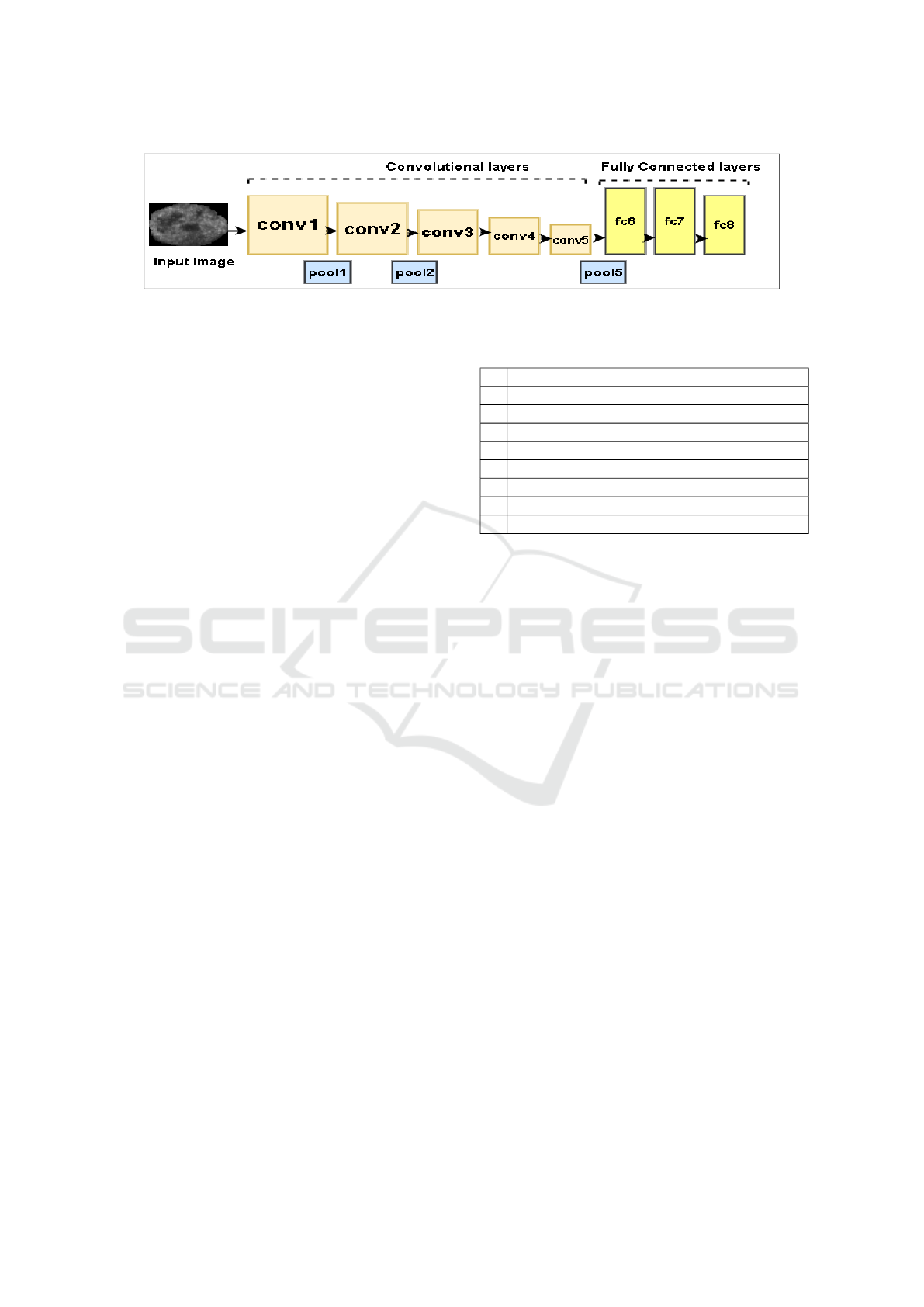
Figure 3: AlexNet architecture.
We now elaborate on the important aspects of our
proposed approach.
2.1 Pre-trained CNN Architecture
Unlike the prior approaches for the mitotic vs non-
mitotic classification task, we propose to use a CNN
based feature representation scheme, in which the
output responses of each layer are used as a generic
feature representation. The idea of using CNN based
features is motivated by its efficacy in various image
processing and pattern recognition tasks (Xu et al.,
2015; Sharif Razavian et al., 2014). We have used a
publicly available pre-trained CNN architecture, i.e.
AlexNet (Krizhevsky et al., 2012), trained on 1.3
million high-resolution images in the LSVRC-2010
ImageNet training set into the 1000 different object
classes. Figure 3 shows the structure of the network.
The network consists of 8 learned layers, including
5 convolutional layers with a kernel size varies from
3 × 3 to 11 × 11 and 3 fully connected layers. Recti-
fied Linear Units (ReLU) is used as a non-linear acti-
vation function at each layer. Maxpooling kernels of
size 3 × 3 are used at the different layers to build ro-
bustness for intra-class variations. We have used the
pre-trained CNN architecture, that is trained on ob-
ject images. Considering the 2D gray level images
involved in the work, we use the 2D CNN. However,
the proposed framework (including the CNN used) is
not restricted to the input image dimension and can
be extended in a straightforward manner for 3D input
images also.
Also involving the visual differences in the two
classes, we believe that the low-level or the higher-
level features representation from such a pre-trained
CNN can still effectively capture the discriminative
information from cell images also. In section 3, we
provide and discuss some activation maps to elaborate
on this point, based on visualization of the feature rep-
resentation. In Table 1, the details of layer types are
given, along with the filter sizes and stride rates.
Table 1: Details in pre-trained AlexNet architecture.
layer Type Size
1 conv1 layer + ReLu 96 × 55 × 55
2 maxpool1 96 × 27 × 27, stride 2
3 conv2 layer + Relu 256 × 27 × 27
4 maxpool2 256 × 13 × 13, stride 2
5 conv3 layer + ReLu 384 × 13 × 13
6 conv4 layer + ReLu 384 × 13 × 13
7 conv5 layer + ReLu 256 × 13 × 13
8 maxpool5 256 × 6 × 6, stride 2
2.2 Layer-wise Features
Importantly, we consider the extraction of the output
responses from different layers of CNN as low-level
features, mid-level features and high level features
representation. Hence, we use the output responses
of layer conv1 with 96×55 × 55 & conv2 with 256 ×
27 × 27 response as low-level feature representation,
conv3 with 384 × 13 × 13 as mid-level feature repre-
sentation and similarly conv4 with 384 × 13 × 13 &
conv5 with 256 × 13 × 13 output responses as high-
level feature representation. Thus, we explore the lay-
ers for which we get a good representation for dis-
criminating the input samples.
2.3 Classification Task
For classification task, we employ the traditional clas-
sifier i.e. Support Vector Machines (SVM). The SVM
classifier can select very few optimal samples (the
support vectors) to build the final model. Arguably,
this aspect can be important in a scenario where we
have less data (as is the case for the undersampling
scenario in this work). Thus, we believe that the SVM
can be a good choice of classifier, as we also later
demonstrate. For SVM classifier, we chose the stan-
dard linear kernel instead of using any non-linear ker-
nel. This is because of one of the purposes of this
work is to gauge the effectiveness of different lay-
ers of CNN features, and a linear classifier would not
transform features in any manner. Indeed, a linear
CNN based Mitotic HEp-2 Cell Image Detection
169
(a) (b) (c)
(d) (e)
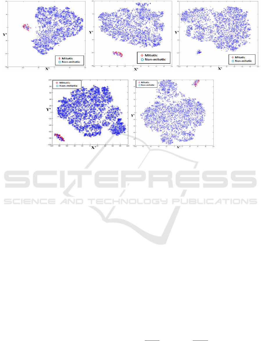
Figure 4: 2-D t-SNE-plot of high dimensional feature representation at (a) conv1, (b) conv2, (c) conv3, (d) conv4, and (e)
conv5 (Better viewed in color or by zooming the images). The high dimensional feature representation is demonstrated in
(X
0
,Y
0
) space.
separation in features is indicated by the t-SNE plots
(Van der Maaten and Hinton, 2008) of Figure 4 .
For comparison, we also perform classification us-
ing the same CNN architecture with Fully Connected
(FC) layers. We treat this as a baseline classifier, and
draw some useful insight from this comparison.
2.4 Data-skew
Considering a large amount of data skew between
both the classes, we apply a well-known data skew
handling techniques of undersampling and oversam-
pling (for the case of the baseline CNN classifier).
In the first case, we undersample the majority class
samples in data space itself. Here, mitotic class im-
ages are the positive images with minority and non-
mitotic is the majority class. Undersampling is done
by randomly removing few samples from the non-
mitotic class and equalizing the samples with the mi-
nority class. We demonstrate that most of our results
are good even with undersampling. In the second
case, an oversampling technique has also been tried
for the same case, where oversampling of minority
class samples are done using data augmentation with
rotation. We rotate images in a range of angles be-
tween 0
◦
to 150
◦
in data space itself. In this case, the
oversampling of minority class is done 40 times.
3 EXPERIMENTS & RESULTS
In this section, we describe about the dataset, experi-
mental details, and results of the proposed approach.
3.1 Dataset Description
To validate our approach, we have used a publicly
available dataset, i.e I3A Task 3 mitotic cell detection
dataset (Vento, ; Foggia et al., 2013). It comprises of
100 mitotic cells and 4228 non-mitotic cells. All cells
are accompanied with a ground truth or mask images.
The mask images are provided to locate the cell nu-
clei region, though we have not used the mask image
in our current work. The mitotic images are annotated
as +1 and non-mitotic mask images as -1.
3.2 Experiment Details
For evaluation, we report the True-Positives (TP) and
False-Positives (FP) accuracy. Mitotic class is con-
sidered as the positive class here. The F-score is also
calculated for the results, which is the harmonic mean
of precision and recall. Here, precision is defined
as
T P
T P+FP
and recall is
T P
T P+FN
and FN denotes False
Negatives.
We report results on a series of experiments that
we conducted on different sets of training, testing and
BIOIMAGING 2018 - 5th International Conference on Bioimaging
170

Table 2: Experimental results of mitotic v/s non-mitotic classification. Here US & OS stand for undersampling and oversam-
pling results respectively.
Layers Training set Validation set Testing set TP acc. FP acc. Precision Recall F-score
(%) (%) (%) (%) (%)
Conv1
30 10 60 87.33 1.23 0.98 0.87 0.92
40 10 50 90.60 1.14 0.98 0.90 0.94
50 10 40 91.50 1.33 0.99 0.91 0.96
Conv2
30 10 60 90.17 1.13 0.99 0.90 0.94
40 10 50 94.80 1.20 0.99 0.95 0.96
50 10 40 95.00 1.24 0.99 0.95 0.97
Conv3
30 10 60 25.90 2.41 0.92 0.26 0.41
40 10 50 35.60 3.62 0.91 0.36 0.52
50 10 40 37.31 3.81 0.91 0.37 0.52
Conv4
30 10 60 98.33 1.14 0.99 0.98 0.98
40 10 50 100 1.07 0.98 1.00 0.99
50 10 40 100 1.08 0.99 1.00 0.99
Conv5
30 10 60 93.6 1.21 0.98 0.93 0.96
40 10 50 98.8 1.21 0.98 0.98 0.98
50 10 40 100 1.21 1.00 1.00 0.99
Pool5
30 10 60 93.60 1.10 0.98 0.93 0.96
40 10 50 99.8 1.19 0.98 0.99 0.98
50 10 40 100 1.10 0.99 1.00 0.99
Baseline-US
30 10 60 68.33 1.02 0.99 0.68 0.81
40 10 50 76 1.04 0.99 0.76 0.8
50 10 40 92.5 1.05 0.99 0.93 0.95
Baseline-OS
30 10 60 95 1.4 0.99 0.95 0.97
40 10 50 98 1.14 0.99 0.98 0.98
50 10 40 80 1.1 0.99 0.8 0.88
validation sets. The dataset is divided into different
ratio of training, validation and testing sets that is
clearly described in Table 2. In our experimentation,
the entire dataset is divided into 3 experimental sets
of 50%, 40% and 30% training sets and 40%, 50%
and 60% testing sets respectively. The average re-
sults are reported over 10 random trials to maintain
the robustness of the experimentation. In this way,
each sample will once include in training, validation
or testing set. In all experimentations, we have used
10% data samples for validation sets, in order to chose
the best model and parameters settings. For classifi-
cation, SVM classifier with standard linear kernel is
used. For this, we have used the well known and effi-
cient LIBLINEAR toolkit (Fan et al., 2008) with best
chosen parameters.
3.3 Results
We report the TP, FP accuracy, precision, recall and
F-score of all experiments in Table 2. The results are
reported in form of low-level, mid and high level fea-
ture representation. As the networks is deep, so we
consider the features from layers 4 and 5 as higher
level features, those from layers 1 and 2 as lower level
features and those from layer 3 as mid-level.
To visually show the discrimination between the
classes and support our experimental results, t-SNE
plots of higher dimensional feature representation of
all the experiments are also presented in 2-dimensions
(better viewed in color) in Figure 4. t-SNE is an
approach to represent high dimensional data in 2-
dimensions (Van der Maaten and Hinton, 2008).
Moreover, we also visualize the activation maps,
i.e. feature maps of conv1 as low-level features,
conv3 as mid-level features and conv5 as high-level
feature representation in Figure 5 (Zeiler and Fergus,
2014), by using a deep visualization toolbox (Yosin-
ski et al., 2015). The feature maps are shown for mi-
totic as well as for one non-mitotic cell class.
We observe that the classification accuracies of
low-level feature representation and high-level repre-
sentation are very high, even with very low amount of
data due to undersampling (which obviates the need
for oversampling in this case). The F-score values are
more than 0.9 in most of the cases. On the other hand,
the mid-level features show a very low accuracy sug-
gesting that these are not discriminative enough.
We discuss more about the layer-wise perfor-
mance along with some observations from the t-SNE
plots and activation maps, and the comparison with
the baseline CNN classifier, in the following subsec-
tions.
CNN based Mitotic HEp-2 Cell Image Detection
171
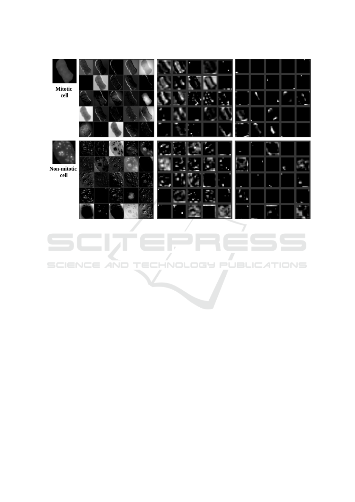
Figure 5: CNN-based feature extraction. Activation maps from Conv1 layer as low-level feature representation (2nd column),
Conv3 as mid-level (3rd column) and Conv5 as high-level feature representation (4th column) are shown.
3.3.1 Conv1 and Conv2: Low-level Feature
Representation
For low-level feature description, we extract the
learned filter responses from conv1. Typically, the
low-level representations exploits the intensity-based
and some texture-based discriminative information.
One can note that the classification results using
conv1 and conv2 features are quite good. This indi-
cates that the low-level intensity variation and texture
information (as also observed in Figure. 1 images)
can be effective for classification. The clear discrimi-
nation between samples is also observed in the t-SNE
plot (Figures. 4(a) and 4(b)).
On the basis of visualization of activation maps
examples from Figure 5 and classification results
from Table 2, we observe that low-level feature rep-
resentation are indeed clearly discriminative and rep-
resent the characteristics well. This is because the
low-level features such as lines, edges, corners and
dots or small blobs etc. are typically common to im-
ages irrespective of their domain. Thus, in this case,
if there is discriminative information at the low-level
such features are able to capture the same, even if the
network is trained on object image data. Hence, we
conclude that the AlexNet architecture, pre-trained on
object images shows the feature representation, in-
cluding the combinations of basic low-level entities
in different sizes, shapes and textures, which are also
quite useful for our classification task.
3.3.2 Conv3: Mid-level Feature Representation
We note the classification accuracies with conv3 fea-
tures are quite low. As implied in some reported
works (Oquab et al., 2014), the mid-level layer may
require some re-training with respect to the cell im-
ages, as the pre-trained architecture is trained on a
very different domain of images. Hence, the con-
textual information and feature representation is quite
different and not discriminative for this domain of im-
ages.
We also note that we are employing a linear classi-
fier, and as observed in the t-SNE plot (Figures. 4(c)),
these features are not linearly separated, and may
need non-linear models for better classification. In
Figure 5, the activation maps of the feature responses
from conv3 are shown. We observe that the features
from conv3 across classes do not differ as clearly as
in the case of low-level features. Thus, many filter
may have irrelevant information, which may reduce
the performance of classifier. Having said that, it is
worth further exploring the interpretation of the mid-
level features in this context.
BIOIMAGING 2018 - 5th International Conference on Bioimaging
172

3.3.3 Conv4, Conv5 and Pool5: High-level
Feature Representation
With regards to the discussion above, this is an inter-
esting case. We observe that the classification accura-
cies with learned features from conv4 and conv5 lay-
ers are very high. As for the low-level features, in this
case too, the t-SNE plot (Figures. 4(d) and 4(e)) show
a clear linear discrimination between the two classes.
Typically, these feature representation is known
to incorporate more semantic information for object
/ scene images. However, for the cell image classifi-
cation case, the images do not seem to have such high
level semantic information, and the activation maps in
Figure 5 seem to support this argument. Thus, while
the activation maps are again not as clearly represen-
tative as those for low-level features, one hypothesis
for the high performance is that the activation maps
are also highly sparse. This could indicate that filter
responses of irrelevant filters (in conv3) might be sup-
pressed in high-level features and only few relevant
filters might activated with discriminative responses.
Again, as for conv3 responses, this is also worth ex-
ploring further to better analyze and interpret the per-
formance of high-level features in this case.
3.4 Comparison with the Baseline CNN
Classifier
Finally, we compare with the baseline CNN classifier
wherein fully connected (FC) layers in the Alexnet
are retrained for classification (Table 2). Note that
both the baseline classifier and one case with the
SVM classifier, operate on the pool5 features. In-
terestingly, in the undersampled case, the baseline
classifier shows a much lower performance than the
SVM classifier, especially with low-amount of train-
ing data. We believe that this is due to over-fitting,
as the amount of data is low. As indicated earlier, the
SVM classifier could be more robust here, as it effec-
tively models the classifier using less number of sam-
ples. Typically, in many applications, the CNN clas-
sifier is trained with oversampled data. In the over-
sampled case, as the data size increases, the baseline
CNN learns better and the accuracy increases. How-
ever, the note that the SVM operating on undersam-
pled data performs equally well.
To the best of our knowledge, there are very few
approaches proposed for this task, and indeed this
is the first work on this dataset. Hence, we do not
provide any comparisons with any other approaches.
However, even in an absolute sense the best results
achieved in this work are quite high and demonstrate
that the approach is very effective to discriminate the
mitotic and non-mitotic class samples.
4 CONCLUSION
In the proposed work, a mitotic cell detection frame-
work for HEp-2 cell images is proposed via learned
feature representation with a pre-trained CNN. We
achieve high quality performance with low-level and
high-level layered features of the architecture. Fur-
thermore, we discuss some useful observations with
respect to the features at various levels, and compari-
son with a baseline CNN. In future, we mean to build
our own classification CNN architecture or re-train
selected layers (transfer learning), which may also
help in achieving better insights.
REFERENCES
Fan, R.-E., Chang, K.-W., Hsieh, C.-J., Wang, X.-R., and
Lin, C.-J. (2008). LIBLINEAR: A library for large
linear classification. J. Mach. Learn. Res., 9:1871–
1874.
Foggia, P., Percannella, G., Soda, P., and Vento, M. (2010).
Early experiences in mitotic cells recognition on HEp-
2 slides. In 2010 IEEE 23rd International Symposium
on Computer-Based Medical Systems (CBMS), pages
38–43.
Foggia, P., Percannella, G., Soda, P., and Vento, M.
(2013). Benchmarking HEp-2 cells classification
methods. IEEE Transactions on Medical Imaging,
32(10):1878–1889.
Gupta, K., Gupta, V., Sao, A. K., Bhavsar, A., and Dileep,
A. D. (2014). Class-specific hierarchical classification
of HEp-2 cell images: The case of two classes. 2014
1st Workshop on Pattern Recognition Techniques for
Indirect Immunofluorescence Images (I3A).
Gupta, V., Gupta, K., Bhavsar, A., and Sao, A. K. (2016).
Hierarchical classification of HEp-2 cell images us-
ing class-specific features. In 6th European Workshop
on Visual Information Processing, EUVIP 2016, Mar-
seille, France, October 25-27, 2016, pages 1–6.
Hobson, P., Lovell, B. C., Percannella, G., Saggese, A.,
Vento, M., and Wiliem, A. (2016). Computer aided
diagnosis for anti-nuclear antibodies HEp-2 images:
Progress and challenges. Pattern Recognition Letters,
82, Part 1:3 – 11. Pattern recognition Techniques for
Indirect Immunofluorescence Images Analysis.
Hobson, P., Lovell, B. C., Percannella, G., Vento, M., and
Wiliem, A. (2014). Classifying anti-nuclear antibod-
ies HEp-2 images: A benchmarking platform. In Pro-
ceedings of the 2014 22nd International Conference
on Pattern Recognition, ICPR ’14, pages 3233–3238,
Washington, DC, USA. IEEE Computer Society.
Iannello, G., Percannella, G., Soda, P., and Vento, M.
(2014). Mitotic cells recognition in HEp-2 images.
Pattern Recognition Letters, 45:136–144.
CNN based Mitotic HEp-2 Cell Image Detection
173

Krizhevsky, A., Sutskever, I., and Hinton, G. E. (2012). Im-
agenet classification with deep convolutional neural
networks. In Advances in Neural Information Pro-
cessing Systems 25, pages 1097–1105. Curran Asso-
ciates, Inc.
Kumar Y, Bhatia A, R. M. (2009). Antinuclear antibodies
and their detection methods in diagnosis of connec-
tive tissue diseases: a journey revisited. Diagnostic
Pathology, 82, Part 1.
Manivannan, S., Li, W., Akbar, S., Wang, R., Zhang, J., and
McKenna, S. J. (2016). An automated pattern recog-
nition system for classifying indirect immunofluores-
cence images of HEp-2 cells and specimens. Pattern
Recognition, 51:12 – 26.
Miros, A., Wiliem, A., Holohan, K., Ball, L., Hobson,
P., and Lovell, B. C. (2015). A benchmarking plat-
form for mitotic cell classification of ANA IIF HEp-2
images. In 2015 International Conference on Digi-
tal Image Computing: Techniques and Applications,
DICTA 2015, Adelaide, Australia, November 23-25,
2015, pages 1–6.
Oquab, M., Bottou, L., Laptev, I., and Sivic, J. (2014).
Learning and transferring mid-level image represen-
tations using convolutional neural networks. In Pro-
ceedings of the 2014 IEEE Conference on Computer
Vision and Pattern Recognition, CVPR ’14, pages
1717–1724, Washington, DC, USA. IEEE Computer
Society.
Percannella, G., Soda, P., and Vento, M. (2011). Mitotic
HEp-2 cells recognition under class skew. In Image
Analysis and Processing – ICIAP 2011: 16th Interna-
tional Conference, Ravenna, Italy, September 14-16,
2011, Proceedings, Part II, pages 353–362.
Sharif Razavian, A., Azizpour, H., Sullivan, J., and Carls-
son, S. (2014). CNN features off-the-shelf: An as-
tounding baseline for recognition. In The IEEE Con-
ference on Computer Vision and Pattern Recognition
(CVPR) Workshops.
Tonti, S., Di Cataldo, S., Macii, E., and Ficarra, E. (2015).
Unsupervised HEp-2 mitosis recognition in indirect
immunofluorescence imaging. In Engineering in
Medicine and Biology Society (EMBC), 2015 37th
Annual International Conference of the IEEE, pages
8135–8138. IEEE.
Van der Maaten, L. and Hinton, G. (2008). Visualizing
high-dimensional data using t-SNE.
Vento, M. Benchmarking HEp-2 mitotic cell detec-
tion dataset, http://nerone.diem.unisa.it/hep2-
benchmarking/dbtools/.
Xu, Z., Yang, Y., and Hauptmann, A. G. (2015). A discrim-
inative CNN video representation for event detection.
In The IEEE Conference on Computer Vision and Pat-
tern Recognition (CVPR).
Yosinski, J., Clune, J., Nguyen, A., Fuchs, T., and Lipson,
H. (2015). Understanding neural networks through
deep visualization. In Deep Learning Workshop, In-
ternational Conference on Machine Learning (ICML).
Zeiler, M. D. and Fergus, R. (2014). Visualizing and under-
standing convolutional networks. In European confer-
ence on computer vision, pages 818–833. Springer.
BIOIMAGING 2018 - 5th International Conference on Bioimaging
174
