Orthogonal Compaction using Additional Bends

Michael J

unger

, Petra Mutzel

and Christiane Spisla

University of Cologne, Cologne, Germany

TU Dortmund, Dortmund, Germany

Keywords:

Orthogonal Compaction, Graph Drawing, Total Edge Length, Bends, Flow-based Compaction.

Abstract:

Compacting orthogonal drawings is a challenging task. Usually algorithms try to compute drawings with small

area or total edge length while preserving the underlying orthogonal shape. We suggest a moderate relaxation

of the orthogonal compaction problem, namely the one-dimensional monotone ﬂexible edge compaction prob-

lem with ﬁxed vertex star geometry. We further show that this problem can be solved in polynomial time using

a network ﬂow model. An experimental evaluation shows that by allowing additional bends we were able to

reduce the total edge length and the drawing area.

1 INTRODUCTION

The compaction problem in orthogonal graph draw-

ing deals with constructing an area-efﬁcient draw-

ing on the orthogonal grid. Every edge is drawn

as a sequence of horizontal and vertical segments,

where the vertices and bends are placed on grid

points. Compaction has been studied in the context

of the topology-shape-metrics approach (Batini et al.,

1986). Here, in a ﬁrst phase a combinatorial embed-

ding is computed that determines the topology of the

layout with the goal to minimize the number of cross-

ings. In the second phase, a dimensionless orthogo-

nal shape of the graph is determined by ﬁxing the an-

gles between adjacent edges and the bends along the

edges. The goal is to minimize the number of bends,

which can be done in polynomial time for a ﬁxed em-

bedding (Tamassia, 1987). In the third phase, metrics

are added to the orthogonal shape. In this context, ﬁrst

the coordinates of vertices and bends are assigned to

grid points so that the given orthogonal shape is main-

tained. Finally, the (orthogonal) compaction problem

asks for a drawing minimizing geometric aestetic cri-

teria, such as the area of the drawing or the total edge

length. The shape is not allowed to change.

Since the orthogonal compaction problem is NP-

hard (Patrignani, 1999), in practice heuristics are used

that ﬁx the x- (or y-, resp.) coordinates and solve

the resulting compaction problem in one dimension.

Given an initial drawing, the one-dimensional com-

paction problem with the goal of minimizing the

height (or width, resp.) of the layout can be trans-

formed to the longest path problem in a directed

acyclic graph. If in addition the total edge length shall

be minimized, the problem can be solved by comput-

ing a minimum cost ﬂow.

The topology-shape-metrics approach aims at

drawings with a small number of crossings, a small

number of bends, and a small drawing area. These

goals are addressed in this order. And indeed, com-

pared with other drawing methods, the number of

crossings and bends is relatively small (Di Battista

et al., 1997). However, the layouts often contain large

areas of white space. It seems that the goal of get-

ting a small drawing area has not been achieved so

far. Consider the drawing in Fig. 1(a) which contains

large areas of white space due to shape restrictions.

By introducing two bends on one of the edges the

drawing area can be reduced drastically. This moti-

vates us to study a compaction problem in which the

shape conditions are relaxed.

This brings us back to the origin of the or-

thogonal compaction problem in VLSI-design (see,

e.g., Lengauer (1990)). In contrast to the compaction

problem considered in graph drawing, even the per-

mutation of wires along the boundary of a component

(and hence, changing the embedding) is allowed.

We suggest a moderate relaxation of the orthogo-

nal compaction problem. More precisely, we suggest

to study the one-dimensional monotone ﬂexible edge

compaction problem with ﬁxed vertex star geometry,

henceforth the Fled-Five compaction problem, which

asks for the minimization of the vertical (horizontal,

resp.) edge length and allows changing the orthogonal

shape of edges, but preserves the x-monotonicity (y-

144

Jünger, M., Mutzel, P. and Spisla, C.

Orthogonal Compaction using Additional Bends.

DOI: 10.5220/0006713301440155

In Proceedings of the 13th International Joint Conference on Computer Vision, Imaging and Computer Graphics Theory and Applications (VISIGRAPP 2018) - Volume 3: IVAPP, pages

144-155

ISBN: 978-989-758-289-9

monotonicity, resp.) of edge segments and prohibits

changing the directions of the initial edge segments

around the vertices (vertex star geometry). We present

a polynomial-time algorithm based on a network ﬂow

model that solves the Fled-Five compaction problem

to optimality. Our computational results show that re-

peated application of Fled-Five compaction in x- and

y-direction is able to reduce the total edge length and

the drawing area at the expense of additional bends.

This paper is organized as follows. We recall the

state of the art in Sect. 2 and some basic deﬁnition

about orthogonal graph drawing and especially the

compaction phase in Sect. 3. We present our new al-

gorithm in Sect. 4 and evaluate it experimentally in

Sect. 5.

(a) (b)

Figure 1: (a) A drawing with large areas of white space due

to shape restrictions. (b) Introducing two additional bends

to one edge of the drawing leads to a smaller drawing.

2 STATE-OF-THE-ART

Patrignani (1999) has shown that planar orthogonal

compaction is in general NP-hard and Bannister et al.

(2012) have given inapproximability results for the

nonplanar case. But for some special cases there ex-

ist polynomial-time algorithms, e.g., if all faces are

of rectangular shape (Di Battista et al., 1999) or if

all faces are so-called turn-regular (Bridgeman et al.,

2000) or have a unique completion (Klau and Mutzel,

1999). Klau and Mutzel (1999) suggested a branch-

and-cut approach to solve an integer linear program

based on extending a pair of constraint graphs.

However, in practice, heuristics are used which it-

eratively ﬁx the x-, and then the y-coordinates, and

solve the resulting one-dimensional compaction prob-

lem. This process is repeated until no further progress

is made. One-dimensional compaction algorithms of-

ten use either network ﬂow techniques or a longest

path method in order to assign integer coordinates to

the vertices, see, e.g., Kaufmann and Wagner (2001)

for an overview. An experimental comparison of pla-

nar compaction algorithms was presented by Klau

et al. (2001).

There has been some work to improve the qual-

ity of a drawing by changing its shape, e.g., F

oßmeier

et al. (1998) or Six et al. (1998). The former uses

shifting and resizing vertices and modiﬁes the shape

of the edges in order to save area and bends, and the

latter may additionally change the topology to im-

prove the drawing. But most compaction algorithms

for planar 4-graphs take as input an orthogonal repre-

sentation and try to produce compact drawings with

respect to that representation. This can lead to an un-

necessarily large drawing area with unused space. Of-

ten better results in terms of area and edge length can

be achieved if the orthogonal shape can be altered, as

we have seen in Fig. 1. On the other hand, it might

be desirable to not change a given drawing too much

in order to preserve the mental map. In some applica-

tions, like layouting data ﬂow diagrams, edges should

start and end at speciﬁc points or sides of the ver-

tices (Sp

onemann et al., 2010). These so-called port

constraints would correspond to ﬁxing the initial edge

segments around vertices (vertex star geometry) in an

orthogonal representation while leaving ﬂexibility to

the edges.

3 NOTATION AND

PRELIMINARY RESULTS

In this section we give basic deﬁnitions and nota-

tions. For more details on orthogonal drawings and

graph drawing in general see, e.g., Di Battista et al.

(1999), Kaufmann and Wagner (2001) or Tamassia

(2013).

3.1 Orthogonal Graph Drawing

For the rest of this paper we restrict ourselves to undi-

rected 4-graphs, i.e. graphs whose vertices have at

most four incident edges. A graph G = (V,E) with

|V | = n and |E| = m is called planar if it admits a

drawing Γ in the plane without edge crossings. Such

a planar drawing of G induces a (planar) embedding,

which is represented by a circular ordered list of bor-

dering edges for every face. The unbounded region of

a planar drawing is called external face.

An orthogonal representation H is an extension

of a planar embedding that gives combinatorial infor-

mation about the orthogonal shape of a drawing. For

every edge we provide information about the bends

encountered while traversing the edge and the angle

formed at vertices by two consecutive edges. If one

of these angles is 270

◦

or 360

◦

we associate with v a

reﬂex corner. An orthogonal representation is called

normalized if it has no bends. An orthogonal grid

Orthogonal Compaction using Additional Bends

145

drawing Γ of G is a drawing in which every edge is

drawn as a sequence of horizontal and vertical edge

segments and every vertex and bend has integer coor-

dinates. Such a drawing induces an orthogonal rep-

resentation H

and a star geometry for every vertex

ﬁxing the directions of the initial line segments of its

incident edges. If an edge ﬁrst turns to the right and

then to the left, or vice versa, we call this a double

bend and the edge segment between these two bends

a middle segment. Every orthogonal representation

can be normalized by replacing all bends in H

with

dummy vertices of degree two, thus adding vertices to

G and Γ.

Since our new approach is based on a network

ﬂow model for one-dimensional compaction, we will

give a brief introduction to minimum cost ﬂows here.

For more information about network ﬂows, see Ahuja

et al. (1993). Let N = (V

) be a directed graph.

Whenever we talk about ﬂows we will call N a net-

work, the members of V

nodes and the members

of E

arcs (in contrast to vertices and edges in an

undirected graph). Every arc a has a lower bound

l(a) ∈ R

≥0

, an upper bound u(a) ∈ R

≥0

∪ {∞}

and a nonnegative cost c(a). A demand b(n) ∈ R

is associated with every node. We call a func-

tion x : A → R

≥0

a ﬂow if x satisﬁes the following

conditions:

capacity constraint:

l(a) ≤ x(a) ≤ u(a) ∀ a ∈ E

(1)

ﬂow conservation:

∑

a=(k,l)

x(a) −

∑

a=( j,k)

x(a) = b(k) ∀ k ∈ V

(2)

A minimum cost ﬂow is a ﬂow x with minimum to-

tal cost c

∑

a∈E

x(a)c(a) under all feasible ﬂows.

The minimum cost ﬂows we are interested in can be

computed in O (|V

3/2

log|V

|) time (Cornelsen and

Karrenbauer, 2012).

3.2 Compaction of Orthogonal

Drawings

We focus on the vertical (orthogonal) compaction

problem that receives as input a planar grid drawing Γ

of a graph G with an orthogonal representation H

and asks for another planar orthogonal drawing Γ

of G realizing H

so that the vertical edge length is

minimized subject to ﬁxed x-coordinates. In the fol-

lowing we describe a ﬂow-based method for vertical

compaction similar to the coordinate assignment al-

gorithm in Di Battista et al. (1999).

Assume we have an initial grid drawing Γ. In

a ﬁrst step we normalize H

resulting in

Γ and H

Then we add vertical visibility edges (so-called dis-

secting edges). We insert a vertical edge connect-

ing each reﬂex corner with the vertex or edge that

is visible in vertical direction, possibly introducing

dummy vertices. This gives us

Γ and

. This way

we eliminate all reﬂex corners and have a represen-

tation with rectangular faces. Now we are ready to

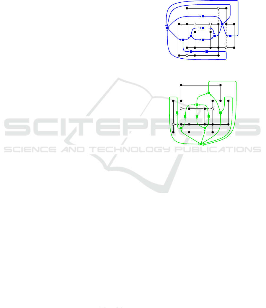
(a)

(b)

Figure 2: The ﬂow networks (a) N

for vertical compaction

and (b) N

for horizontal compaction. White vertices are

dummy vertices and dashed edges are dummy edges.

construct the network N

for vertical compaction. For

each face f in representation

we add a node n

to N

with demand b(n

) = 0 and for every vertical

edge e with left face f

and right face f

we insert an

arc a

= (n

) with lower bound l(a

) = 1 and up-

per bound u(a

) = ∞. If e is a dummy edge a

gets

zero cost, otherwise a cost of one. See Fig. 2 for an

example.

Suppose we have computed a feasible ﬂow. Now

a unit of ﬂow corresponds to one unit of vertical edge

length. The x-coordinates remain unchanged. The ca-

pacity constraint assures that every edge gets a min-

imum length of one and the ﬂow conservation con-

straint guarantees that every face is drawn as a proper

rectangle. Finally, the visibility edges and dummy

vertices can be removed.

Lemma 1. The above algorithm solves the vertical

compaction problem to optimality.

IVAPP 2018 - International Conference on Information Visualization Theory and Applications

146

Proof. In the vertical compaction problem we have

to preserve the vertical visibility properties of Γ in

order to avoid overlapping graph elements. This is

achieved by the newly added visibility edges. Be-

cause of the one-to-one correspondence of vertical

length of an edge segment in the resulting drawing Γ

and the amount of ﬂow carried by a non-zero-cost arc

∈ N

, the result of the minimum cost ﬂow gives

us a minimal vertical length assignment.

4 THE FLED-FIVE COMPACTION

APPROACH

In this section we study the following relaxation

of the one-dimensional compaction problem called

the monotone ﬂexible edge compaction problem with

ﬁxed vertex star geometry (Fled-Five compaction

problem). For vertical compaction it is deﬁned as fol-

lows: Given a planar grid drawing Γ of a 4-graph G

with an orthogonal representation H

, compute an-

other planar grid drawing of G that minimizes the

vertical edge length subject to ﬁxed x-coordinates in

which all horizontal edge segments of Γ are drawn

x-monotonically and the vertex star geometry for all

vertices as well as the planar embedding is main-

tained.

In contrast to the classical compaction problem,

it is not required here to realize the entire orthogonal

representation, but only the local geometric surround-

ing of each vertex. The ﬁxed x-coordinates and the

x-monotonicity prohibits the lengthening of the total

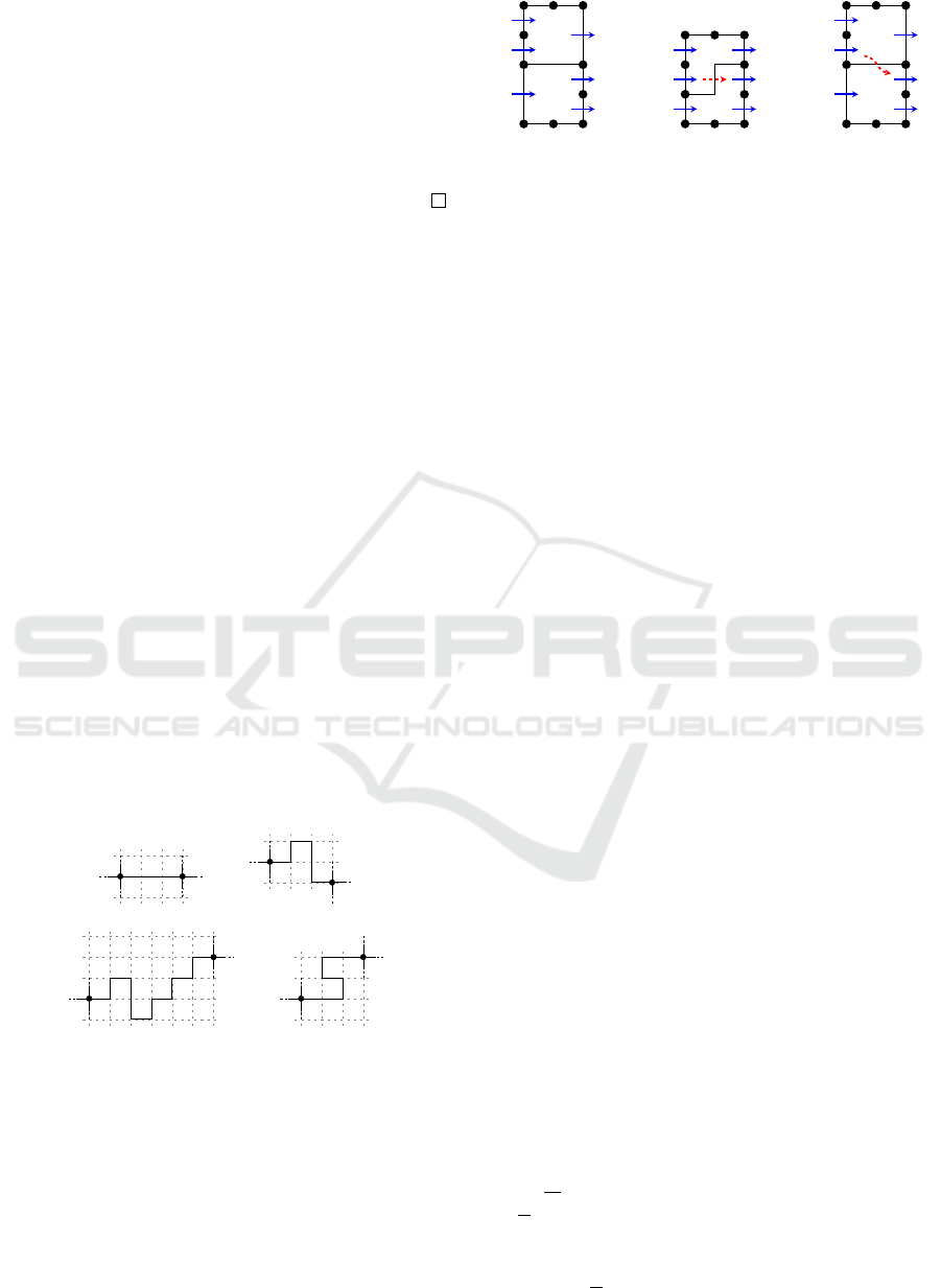
horizontal edge length (see Fig. 3).

(a) (b)

Figure 3: Modiﬁcations in Fled-Five. (a) The original edge

of length three. (b) Modiﬁcation allowed in Fled-Five.

(d) not allowed, because x-monotonicity is violated.

We adapt the network ﬂow approach described in

Sect. 3.2. But now we are able to introduce or remove

double bends of certain edges in order to improve the

vertical edge length. We illustrate the concept by the

following example. Figure 4(a) shows an optimally

compacted drawing with respect to its orthogonal rep-

(a) (b) (c)

Figure 4: A graph and the arcs of the corresponding ﬂow

network (a,b) of the traditional algorithm and (c) in our al-

gorithm.

resentation. The blue arcs show the arcs of the verti-

cal compaction network (compare Fig. 2). For better

readability we omitted the network nodes belonging

to the faces. In Fig. 4(b), the same graph is shown,

but with a different orthogonal representation. The

new double bend in the middle edge leads to a smaller

drawing. In this drawing it is possible to send ﬂow be-

tween the two internal faces, since they are separated

by a vertical edge segment. In the corresponding ﬂow

network there is a new network arc (red, dashed) con-

necting the upper and the lower face. This leads to

the key idea of our approach. Introducing arcs in the

vertical ﬂow network between horizontally separated

face nodes enables us to shift ﬂow between them and

therefore exchange vertical edge length at the expense

of a double bend (see Fig. 4(c)). We can also reverse

this thought. If there is an unnecessary double bend

we can get rid of it by not sending ﬂow over the arc

corresponding to its middle segment and thus remov-

ing the middle segment from the drawing.

But we have to be careful here. First, we are com-

pacting in vertical direction, so we cannot change the

x-coordinates. If an edge has a double bend, it needs

to have a horizontal expansion of at least two. Thus

we will not consider edges of length one as possible

candidates for getting a double bend. Second, adding

a double bend to e introduces two reﬂex corners, one

in both adjacent faces of e. Two double bends may

even cause an edge overlap, see Fig. 5(a). We need to

ensure that the computed ﬂow corresponds to a feasi-

ble drawing. Therefore we will treat each grid point

along an edge that could be part of a double bend

as a potential reﬂex corner, which we will eliminate

by dissecting. We will now describe the algorithm

in detail.

Our algorithm works in three phases: dissection,

computation of a minimum cost ﬂow and transform-

ing the ﬂow into a new drawing. First we normalize

to H

. For dissection we split the horizontal edges

of Γ by placing an artiﬁcial bend vertex on every in-

ner grid point of an horizontal edge. The bend ver-

tices may later be transformed to double bends. Then

we dissect Γ as described in Sect. 3 and treat every

Orthogonal Compaction using Additional Bends

147

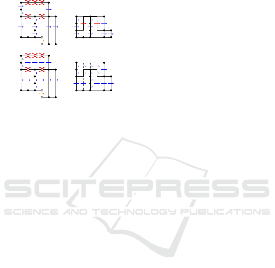
2 2

(a)

2 2 2 2

1 1

(b)

Figure 5: Input graph with modiﬁed ﬂow network and a

minimum cost ﬂow (all unlabeled arcs carry one unit of

ﬂow) with the resulting drawing (a) without additional dis-

secting edges and (b) including them. The bold edge in (a)

indicates an edge overlap and the grey vertices result from

normalization, the white vertices in (b) are bend vertices.

Dissecting edges are indicated in (b).

bend vertex as a reﬂex corner in its adjacent faces (see

Fig. 5(b)). That means, we may dissect the drawing

in vertical stripes of unit length. Doing so, we solve

both of the problems mentioned above. Since we con-

sider only edges of length at least two, we guarantee

that the edge will be long enough for a double bend

and by inserting the visibility edges we keep the ver-

tical separation of graph elements intact. This results

in the extensions

Γ and

and

Observation 1. After this dissection method the num-

ber of vertices and edges in

G is O(A), where

A = h

· w

and h

) is the height (width) of Γ.

Next we construct the network from Sect. 3.2. Ad-

ditionally to the already introduced arcs (straight blue

arcs in Fig. 5) we add two arcs a

↑

and a

↓

for every

bend vertex (curved, red arcs in Fig. 5). Notice that

every such bend vertex v has four adjacent faces, one

at the lower and upper left and right. If it lies on the

external face, two of the adjacent faces may coincide.

Arc a

↑

goes from the lower left face of v to its up-

per right face and a

↓

goes from the upper left to the

lower right face. Flow on one of these arcs will lead

to a double bend in the edge segment of G that is split

by v. The lower bound of these arcs is zero, the upper

bound is set to inﬁnity and the cost is one. For every

edge e ∈

G that is a middle segment in G we decrease

the lower bound of its arc a

to zero, since this is a

vertical edge segment, that we may delete (dashed,

orange arc in Fig. 5).

After computing a minimum cost ﬂow in this net-

work, we interpret the result in the following way: For

every vertical edge e of

G we translate the amount of

ﬂow on the arc a

of N

to the length of e. Let a

↑

be an arc corresponding to a bend vertex v carrying k

units of ﬂow. Let e be the split horizontal edge and

the x-coordinate of v. Then e will start at its left

endpoint in horizontal direction, bend downwards at

x-coordinate x

, proceed for k units in y-direction and

then continue to the right to its other endpoint. If we

deal with an arc of the form a

↓

the corresponding edge

will do an upward bend at x

. Let e

∈

G be an edge

that corresponds to a middle segment and let a

be the

corresponding arc. If a

carries no ﬂow we do not as-

sign any vertical length to e

, hence the double bend to

which e

belongs collapses. Notice that ﬂow on every

non-zero-cost arc corresponds to vertical edge length.

Theoretically, it is possible that both a

↑

and a

↓

carry

ﬂow in a feasible, but not optimal, solution. In this

case we can always augment the ﬂow in a way that

at most one of a

↑

or a

↓

carries ﬂow. Finally, we re-

move all dummy edges and vertices. See Fig. 5 for an

example and Algorithm 1 for pseudocode.

Let us assume that the width and height of Γ are

bounded by the number of its vertices and bends. Oth-

erwise there would be a grid line without any vertex

or bend on it. We can delete such grid lines iteratively

until we reach our bound.

Theorem 1. Let Γ be a planar grid drawing of a 4-

graph G with an orthogonal representation H

. Let ¯n

be the number of vertices and bends of Γ. Then the

above described extended network-based compaction

algorithm takes O ( ¯n

log ¯n) time and solves the verti-

cal Fled-Five compaction problem to optimality.

Proof. Because of the visibility edges we will main-

tain visibility properties of Γ. Every vertical edge seg-

ment of G that is not a middle segment gets a mini-

mum length of one due to the lower bound of the cor-

responding arc in N

. Every bend vertex can safely be

turned to a double bend if its corresponding arc carries

ﬂow, since we add visibility edges to the top and bot-

tom of it. By this modiﬁcation we do not change the

vertex star geometry of Γ, because bend vertices are

not part of G. Every middle segment can be removed

if there is no ﬂow on the corresponding arc. Because

its edge e ∈ Γ has a horizontal expansion of at least

two, e will still have a proper length and due to the

dissection phase visibility properties are maintained.

This modiﬁcation also does not affect the vertex star

geometry of Γ, since a middle segment is not adjacent

to a vertex of G. So every face will have a rectangu-

lar shape, no matter what modiﬁcation we apply, and

due to ﬂow conservation every face and thus the entire

graph is drawn consistently. Similar to Lemma 3.2 the

IVAPP 2018 - International Conference on Information Visualization Theory and Applications

148

Input : orthogonal drawing Γ

Output: optimal solution Γ

to the Fled-Five

compaction problem

Γ ← normalize(Γ);

Γ ← addBendVerticesAndVertVisEdges(Γ);

// construct network N

for every face f do

N ← node n

;

demand[n

]=0;

for every vertical edge e do

node n1 = leftFaceNode(e);

node n2 = rightFaceNode(e);

if isMidSegment(e) then

lowerBound[a

]=0;

else lowerBound[a

]=1;

upperBound[a

]=∞;

if isVisEdge(e) then cost[a

] = 0;

else cost[a

]=1;

for every bend vertex v do

node n1 = lowerLeftFaceNode(v);

node n2 = upperRightFaceNode(v);

N ← arc a

↑

= (n1,n2);

lowerBound[a

↑

]=0; upperBound[a

↑

]=∞;

cost[a

↑

]=1;

node n3 = upperLeftFaceNode(v);

node n4 = lowerRightFaceNode(v);

N ← arc a

↓

= (n3,n4);

lowerBound[a

↓

]=0; upperBound[a

↓

]=∞;

cost[a

↓

]=1;

// compute length assignment

x ← computeMinimumCostFlow(N);

for every vertical edge e do

length(e) ← x(networkArc(e));

for every bend vertex v do

edge e ← horizontalEdge(v);

int xc ← xCoordinate(v);

if x(a

↑

) 6= 0 then

addDownwardMidSegment(e,xc,x(a

↑

));

if x(a

↓

) 6= 0 then

addUpwardMidSegment(e, xc,x(a

↓

));

← RemoveBendVerticesAndVisEdges(

Γ);

Algorithm 1: verticalFledFive.

length of vertical segments of Γ

is equal to the cost

of the computed minimum cost ﬂow. Since the initial

drawing can be interpreted as a feasible ﬂow, we get a

drawing Γ

with total edge length less or equal to that

of Γ. The horizontal edge segments maintain their x-

monotonicity, because we only add vertical segments

to the drawing. Hence the horizontal edge lengths and

the x-coordinates of the vertices in Γ stay the same.

Because the minimum cost ﬂow gives us a minimal

vertical length assignment we have an optimal solu-

tion for the vertical Fled-Five compaction problem.

For the running time we ﬁrst consider the dissec-

tion phase. By Observation 1 we end up with O(¯n

)

vertices. For inserting dummy edges based on visibil-

ity properties we can use a sweep-line algorithm that

runs in O ( ¯n

log ¯n) time in our case. The construc-

tion of the ﬂow network runs in linear time in the size

G. The network is planar and has O( ¯n

) nodes.

For planar ﬂow networks with n nodes and O(n) arcs

there exists a O(n

3/2

logn) time algorithm for com-

puting a minimum cost ﬂow (Cornelsen and Karren-

bauer, 2012). Therefore we have a total running time

of O( ¯n

log ¯n).

4.1 Short Remarks

Running Time. The cubic part of the running time

comes from the possibly quadratic number of bend

vertices and dissecting edges. So if we restrict the

number of bend vertices to be linear, we can decrease

the running time to O( ¯n

3/2

log ¯n).

Controlling the Number of New Bends. Although

the above compaction approach may reduce the to-

tal edge length, the number of bends in the resulting

drawing may increase. A possible approach to control

the number of new bends could be to bound the num-

ber of speciﬁc arcs used by a feasible ﬂow. This is

known as the binary case of the budget-constrained

minimum cost ﬂow problem for which Holzhauser

et al. (2016) showed strong NP-completeness. In fact,

in this model we have no other control over the num-

ber of additional bends than restricting the number of

bend vertices. Each such vertex can generate two new

bends. By assigning higher cost to arcs a

↑

and a

↓

becomes more unlikely for these arcs to carry much

ﬂow, but it does not limit its number used by the ﬂow.

It makes no difference in terms of total cost if we

send, e.g., 10 units of ﬂow over a

↑

or one unit of

ﬂow over 10 such arcs, while the former produces two

bends and the latter 20 bends.

Extensions to Other Models. While in a drawing

model for 4-graphs a node occupies exactly one grid

point, there are other models for drawing graphs with

maximum degree greater four, e.g., the Kandinsky

model (F

oßmeier and Kaufmann, 1995), where es-

sentially nodes spread over several grid points (big

nodes) or the quasi-orthogonal model (J

unger et al.,

2004), where edges are allowed to leave the grid

around vertices. Our approach can be extented to

Orthogonal Compaction using Additional Bends

149

10-50 51-100 101-150 151-200 200-314

decrease in %

nodes

total

max

area

100

200

300

400

500

600

700

800

10-50 51-100 101-150 151-200 200-314

increase in %

nodes

bends

time per iteration

time

vis. edges

(a)

-15

-10

-5

40-100 101-200 201-300 301-400 401-500

decrease in %

nodes

total

max

area

100

120

140

160

40-100 101-200 201-300 301-400 401-500

increase in %

nodes

bends

time per iteration

time

vis. edges

(b)

40-100 101-200 201-300 301-400 401-500

decrease in %

nodes

total

max

area

100

150

200

250

300

40-100 101-200 201-300 301-400 401-500

increase in %

nodes

bends

time per iteration

time

vis. edges

(c)

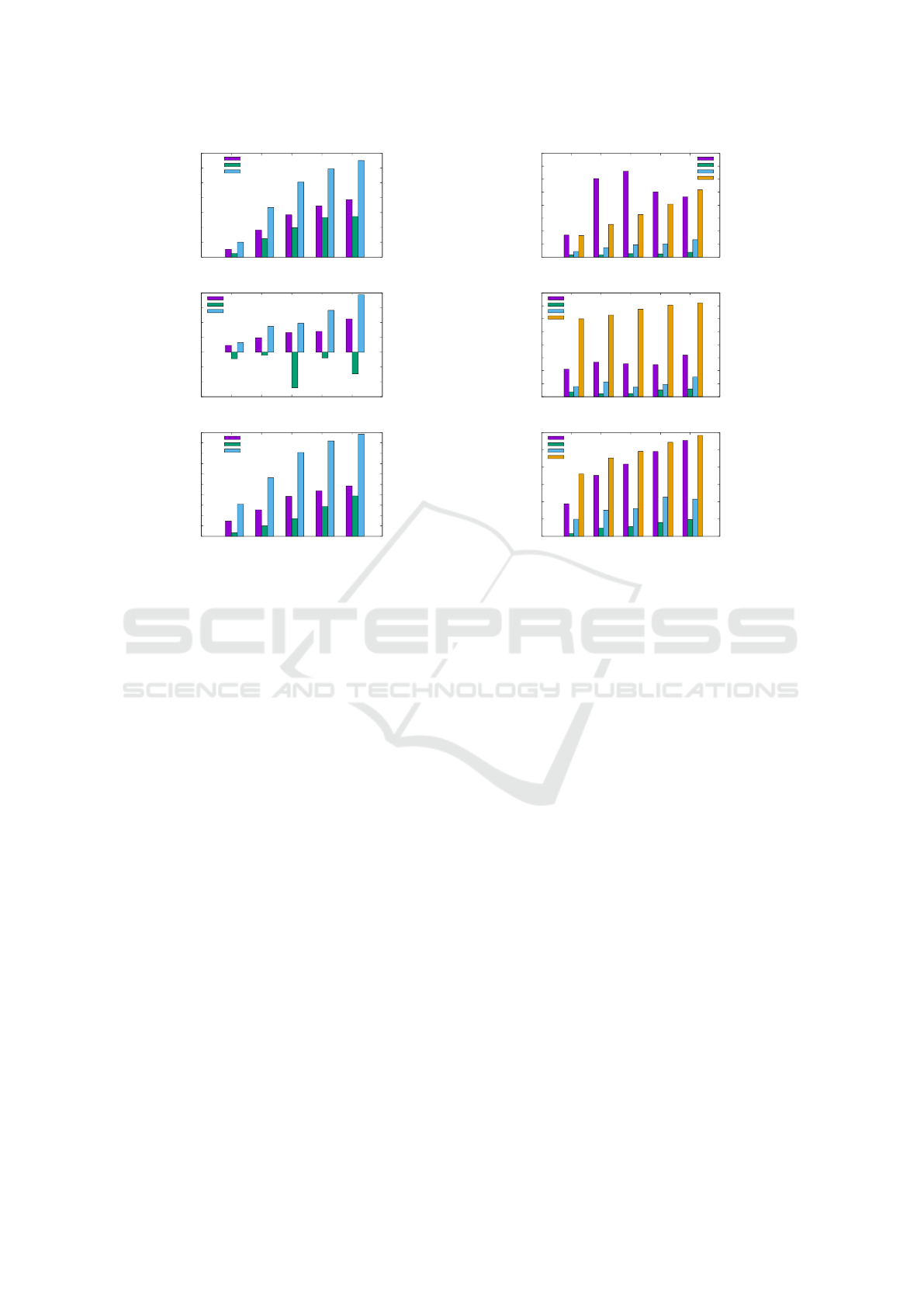
Figure 6: Average change of the total edge length, the maximum edge length, the area, the number of bends, the time per

iteration, the total running time and the number of visibility edges from TRAD to FF in percent for (a) the Rome graphs, (b)

the quasi trees, and (c) the biconnected graphs.

these models in a straightforward way by modeling

big nodes as rectangular faces of suitable size for all

the incident edges and prohibit changing the shape of

the dummy edges that participate in these faces. Since

in the quasi-orthogonal model, until the last step of

actual drawing, high-degree nodes are also handled

as faces, the extension works for this model as well.

5 EXPERIMENTAL EVALUATION

In this section we evaluate our algorithm FF focusing

on the total edge length and area improvement. Klau

et al. (2001) compared 12 compaction heuristics that

maintain the orthogonal representation and we chose

the best of these traditional heuristics (T2FL in Klau

et al. (2001)), which we call TRAD, for comparison

in order to demonstrate the beneﬁt of slightly chang-

ing the orthogonal shape. This method was within

one percent of the optimal value for practical in-

stances. We refrain from comparing to improvement

algorithms like the 4M algorithm (F

oßmeier et al.,

1998) or the reﬁnement method from Six et al. (1998)

since they change the vertex star geometry, the topol-

ogy and even vertex sizes. The moving operation of

the 4M algorithm is the only operation that ﬁts our

model, but would not change any layout generated by

a ﬂow-based compaction algorithm. The only appli-

cable modiﬁcation from Six et al. (1998) (superﬂu-

ous bends) does not have an impact on bend minimal

drawings that we use as input.

The algorithms were implemented in C++ using

the OGDF library (Chimani et al., 2013). For both

algorithms we start with a bend minimal orthogonal

representation. For TRAD we apply a constructive

compaction method, that transforms the orthogonal

representation into a turn-regular one and then runs

a ﬂow-based coordinate assignment in order to get

a feasible planar grid drawing. Then we repeatedly

apply horizontal and vertical compaction steps with

a ﬂow-based improvement heuristic until no further

improvement can be achieved, see heuristic T2FL in

Klau et al. (2001). For FF we use the same con-

structive heuristic and then apply the modiﬁed ﬂow

technique from Sect. 4 with a cost of one for the net-

work arcs causing double bends to achieve best possi-

ble shortening, also repeatedly in horizontal and ver-

tical direction. Recall that although both approaches

are optimal for the one-dimensional compaction prob-

lems, repeated application of horizontal and verti-

cal compaction steps does in general not lead to

drawings with optimal total edge length for the two-

IVAPP 2018 - International Conference on Information Visualization Theory and Applications

150

200

400

600

800

1000

1200

1400

1600

1800

2000

0 100 200 300 400 500

total edge length

nodes

TRAD

(a)

1000

2000

3000

4000

5000

6000

0 100 200 300 400 500

area

nodes

TRAD

(b)

100

0 100 200 300 400 500

maximum edge length

nodes

TRAD

(c)

100

120

140

160

180

200

0 100 200 300 400 500

bends

nodes

TRAD

(d)

0.5

1.5

2.5

0 100 200 300 400 500

time per iteration in seconds

nodes

TRAD

(e)

0 100 200 300 400 500

total running time in sec.

nodes

TRAD

(f)

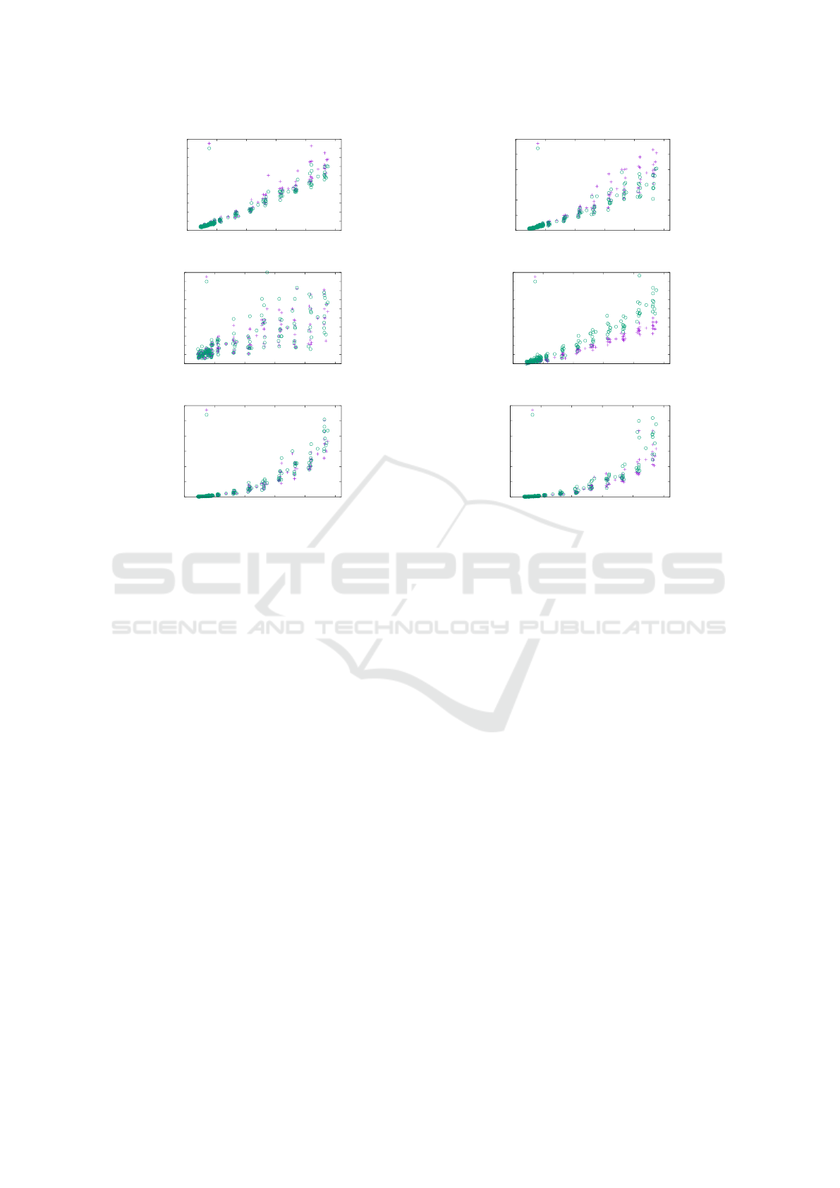
Figure 7: Absolute results of TRAD and FF for the quasi-trees: (a) total edge length, (b) area, (c) maximum edge length, (d)

number of bends, (e) time per iteration, (f) total running time.

dimensional compaction problems. Notice also that

due to the alternating repetitions in FF the monotonic-

ity of edge segments may no longer be maintained.

We state the following hypotheses regarding the

results of our new approach FF compared to those of

TRAD:

(H1) The total edge length and therefore the area

of the drawings will decrease. We will also

examine the change of the maximum edge

length. It is hard to predict the behaviour, be-

cause on the one hand adding a double bend

lengthens an edge, but it could also lead to

shorter edges in other places.

(H2) The number of bends will rise signiﬁcantly.

(H3) Although there will be many more dissecting

edges, the running time will not increase dras-

tically.

We tested our algorithm on three test suites. The

standard benchmark set called Rome graphs intro-

duced in Di Battista et al. (1997) consists of about

11,000 real-world and real-world like graphs with

10 to 100 vertices. The second set of graphs are

quasi-trees which are known to be hard to compact.

They have already been used in the compaction liter-

ature (e.g., Klau et al. (2001), Klau (2002)). From

this, we selected a subset of 155 graphs with 40

to 450 vertices. The last set consists of 240 ran-

domly generated biconnected planar 4-graphs with

40 to 500 vertices. All used graphs were, if neces-

sary, initially turned into planar 4-graphs by planariz-

ing them with methods of OGDF and replacing ver-

tices with k > 4 outgoing edges with faces of size k.

This results in graph sizes of up to 314 vertices for

the Rome test suite and up to 475 vertices for the

quasi-trees before the orthogonalization step. The in-

put instances are available on https://ls11-www.cs.tu-

dortmund.de/mutzel/compaction. All tests were run

on an Intel Xeon E5-2640v3 2.6GHz CPU with 128

GB RAM.

(H1) Figure 6 shows the average decrease of the to-

tal and maximum edge length as well as of the area in

percent. In all three graph classes the total edge length

as well as the area has improved. We were able to de-

crease the total edge length by up to 36.1% and the

area by up to 68.7%. In general, larger graphs allow a

larger improvement. It turned out that for the majority

of the instances we were also able to reduce the maxi-

mum edge length. Only for the quasi-trees the longest

edges produced by FF are longer on average. But in

general the results are mixed, reaching from a length-

ening by 87.5% to a shortening by 58.1%. Figures 7,

Orthogonal Compaction using Additional Bends

151

500

1000

1500

2000

2500

0 50 100 150 200 250 300

total edge length

nodes

TRAD

(a)

500

1000

1500

2000

2500

3000

0 50 100 150 200 250 300

area

nodes

TRAD

(b)

100

120

0 50 100 150 200 250 300

maximum edge length

nodes

TRAD

(c)

100

150

200

250

0 50 100 150 200 250 300

bends

nodes

TRAD

(d)

0.5

1.5

2.5

0 50 100 150 200 250 300

time per iteration in seconds

nodes

TRAD

(e)

0 50 100 150 200 250 300

total running time in sec.

nodes

TRAD

(f)

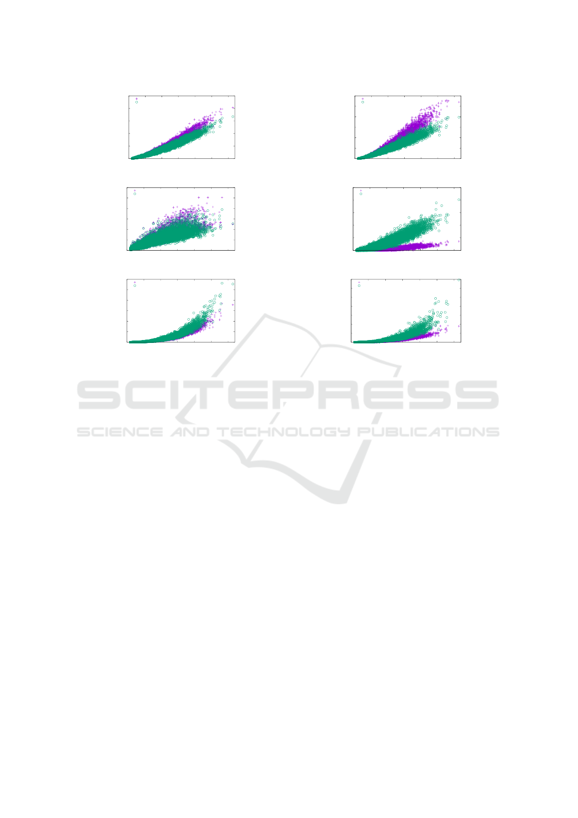
Figure 8: Absolute results of TRAD and FF for the Rome graphs: (a) total edge length, (b) area, (c) maximum edge length,

(d) number of bends, (e) time per iteration, (f) total running time.

8 and 9 (a) - (c) show absolute values for the total

edge length, the area and the maximum edge length

measured for the three graph classes.

(H2) Figure 6 displays the average increase of the

number of bends. If an instance had no bends af-

ter TRAD, we use the number of bends after FF as

relative increase to take also these instances into ac-

count for computing the average increase of bends.

As expected the drawings produced by FF have many

more bends, especially for the Rome graphs. In one

of the worst cases the number of bends went up from

zero to 72. Although the relative increase of bends

is very high, the average number of bends per edge

in the drawings produced by FF is 0.18 for the Rome

graphs, 0.13 for the quasi trees and 0.30 for the bi-

connected graph, respectively. The highest ratio over

all instances is 0.52. Recall, that we started with

bend minimal orthogonal representations. Figures 7,

8 and 9 (d) show the absolute values for the number

of bends measured for the test graphs. Figure 10 gives

the relation between the number of invested bends

and the improvement in terms of area and total edge

length for the biconnected graphs. The data for the

other two graph classes can be found in J

unger et al.

(2017). Figure 11 plots the relation between the num-

ber of bends and the number of edges.

As mentioned before, we cannot limit the num-

ber of bends added by FF, but we decrease the like-

lyhood to send ﬂow over an arc of the form a

↑

or a

↓

by assigning higher costs to these arcs. We evalu-

ated the number of additional bends, the area and to-

tal edge length for different arc costs on the subset

of the Rome graphs with 100 to 150 vertices. These

instances showed the greatest increase regarding the

number of bends. Since we focus on the impact of

the arc cost here, we apply only one compaction step

in each direction. As expected the number of new

bends as well as the achieved improvement in terms

of area and total edge length compared to TRAD de-

creases with increasing arc costs, see Fig. 12. With a

slightly higher arc cost we can reduce the number of

additional bends without drastically affecting the area

and total edge length improvement. The average rela-

tive increase of bends went down from 663.7% for an

arc cost of one to 324.6% for an arc cost of two and

234.3% for an arc cost of three. The average improve-

ment of area (total edge length) is 24.7% (13.8%),

22.5% (11.4%) and 20.5% (10.2%), respectively. The

differences between higher arc costs in terms of addi-

tional bends become smaller. The data regarding the

number of bends scatter over a wide range (notice the

different scale on the right in Fig. 12 for the change

of bends), especially for low arc cost, therefore it is

IVAPP 2018 - International Conference on Information Visualization Theory and Applications

152

1000

2000

3000

4000

5000

6000

0 100 200 300 400 500

total edge length

nodes

TRAD

(a)

2000

4000

6000

8000

10000

12000

14000

0 100 200 300 400 500

area

nodes

TRAD

(b)

100

120

140

160

180

200

0 100 200 300 400 500

maximum edge length

nodes

TRAD

(c)

100

150

200

250

300

350

0 100 200 300 400 500

bends

nodes

TRAD

(d)

0 100 200 300 400 500

time per iteration in seconds

nodes

TRAD

(e)

100

120

0 100 200 300 400 500

total running time in sec.

nodes

TRAD

(f)

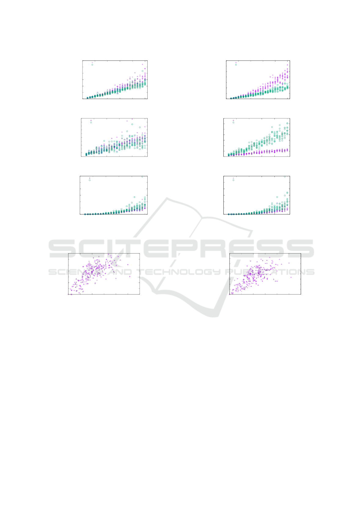
Figure 9: Absolute results of TRAD and FF for the biconnected graphs: (a) total edge length, (b) area, (c) maximum edge

length, (d) number of bends, (e) time per iteration, (f) total running time.

0 100 200 300 400 500 600

decrease of area in %

increase of bends in %

(a)

0 100 200 300 400 500 600

decrease of tot. edge length in %

increase of bends in %

(b)

Figure 10: Relation between additional bends and (a) improvement of area and (b) total edge length for the biconnected

graphs.

hard to determine which arc cost is suitable to keep

the number of additional bends low, but still yields

good geometric results.

(H3) We measured the total running time and the

number of performed compaction iterations. For bet-

ter comparison we also display the running time per

iteration, because FF tends to do more iterations. The

reason for that is that a compaction step of FF changes

the drawing and therefore the ﬂow network of the next

step more signiﬁcantly, leading to more new possibil-

ities in compacting. The right side of Figure 6 dis-

plays the average increase of the running time and the

number of visibility edges. In all cases the number

of additional dissecting edges has increased signiﬁ-

cantly. The running time per iteration has also in-

creased, but not more than 50% on average. Only

for 252 instances of the Rome graphs and one bicon-

nected graph the running time per iteration has more

than doubled.

The results support the hypotheses. Our new ap-

proach is able to improve the drawing area and the to-

tal edge length by introducing additional bends. Fig-

ure 13 shows two examples drawn with TRAD and FF,

respectively.

6 CONCLUSION

We have presented a new compaction heuristic for or-

thogonal graph drawing that alters the orthogonal rep-

Orthogonal Compaction using Additional Bends

153

100

150

200

250

300

350

0 100 20 0 300 400 5 00 600

bends

edges

f(x)=x

(a)

100

150

200

250

300

350

0 100 200 300 400 50 0 600 700

bends

edges

f(x)=x

(b)

100

150

200

250

300

350

0 100 200 300 400 500 600 700 800

bends

edges

f(x)=x

(c)

Figure 11: Number of bends in the drawings produced by FF for (a) the Rome graphs, (b) the quasi trees and (c) the bicon-

nected graphs.

1 2 3 4 5 6 7 8 9 10

200

400

600

800

1000

decrease of area

and edge length in %

increase of bends in %

arc cost

bends

area

edge length

Figure 12: Relative change of the number of bends, area

and total edge length with increasing arc costs for a subset

of the Rome graphs. The whiskers cover 90% of the data,

no outliers are depicted for better readability.

resentation. We were able to reduce the total edge

length and drawing area, but at the expense of addi-

tional bends. Unfortunately, in our model we have no

control over the number of bends added, but if the fo-

cus of interest lies on area and edge length, the results

show a very positive effect. Future research could fo-

cus on studying the trade-off between bends and area

or bends and total edge length as a bicriteria optimiza-

tion problem.

ACKNOWLEDGEMENTS

This work was supported by the DFG under the

project Compact Graph Drawing with Port Con-

straints (DFG MU 1129/10-1). We would like to

thank Gunnar Klau for providing us with most of our

test instances and anonymous reviewers for helpful

remarks on a previous version of this paper. We also

gratefully acknowledge helpful discussions with Mar-

tin Gronemann, Sven Mallach, and Daniel Schmidt.

REFERENCES

Ahuja, R. K., Magnanti, T. L., and Orlin, J. B. (1993). Net-

work Flows: Theory, Algorithms, and Applications.

Prentice-Hall, Inc., Upper Saddle River, NJ, USA.

Bannister, M. J., Eppstein, D., and Simons, J. A. (2012). In-

approximability of orthogonal compaction. J. Graph

Algorithms Appl., 16(3):651–673.

(a)

(b)

(c)

(d)

Figure 13: Biconnected graph with 220 vertices and 304

edges and Rome graph with 55 vertices and 66 edges (af-

ter planarization and expanding high degree vertices): (a)

TRAD: total edge length 1459, area 3060, bends 31 (b) FF:

total edge length 1107, area 1320, bends 133 (c) TRAD: total

edge length 168, area 240, bends 1 (d) FF: total edge length

140, area 140, bends 13. Edges with additional bends are

red.

Batini, C., Nardelli, E., and Tamassia, R. (1986). A layout

algorithm for data ﬂow diagrams. IEEE Transactions

on Software Engineering, SE-12(4):538–546.

Bridgeman, S. S., Di Battista, G., Didimo, W., Liotta, G.,

Tamassia, R., and Vismara, L. (2000). Turn-regularity

and optimal area drawings of orthogonal representa-

tions. Comput. Geom., 16(1):53–93.

Chimani, M., Gutwenger, C., J

unger, M., Klau, G. W.,

Klein, K., and Mutzel, P. (2013). The Open Graph

Drawing Framework (OGDF). In Tamassia, R., edi-

tor, Handbook of Graph Drawing and Visualization,

chapter 17, pages 543–569. CRC Press.

Cornelsen, S. and Karrenbauer, A. (2012). Acceler-

ated bend minimization. J. Graph Algorithms Appl.,

IVAPP 2018 - International Conference on Information Visualization Theory and Applications

154

16(3):635–650.

Di Battista, G., Eades, P., Tamassia, R., and Tollis, I. G.

(1999). Graph Drawing: Algorithms for the Visual-

ization of Graphs. Prentice-Hall, Upper Saddle River,

NJ, USA.

Di Battista, G., Garg, A., Liotta, G., Tamassia, R., Tassi-

nari, E., and Vargiu, F. (1997). An experimental com-

parison of four graph drawing algorithms. Comput.

Geom., 7:303–325.

oßmeier, U., Heß, C., and Kaufmann, M. (1998). On im-

proving orthogonal drawings: The 4m-algorithm. In

Whitesides, S., editor, Graph Drawing, 6th Interna-

tional Symposium, GD’98, Proceedings, volume 1547

of LNCS, pages 125–137. Springer.

oßmeier, U. and Kaufmann, M. (1995). Drawing high

degree graphs with low bend numbers. In Bran-

denburg, F., editor, Graph Drawing, Symposium on

Graph Drawing, GD ’95, Proceedings, volume 1027

of LNCS, pages 254–266. Springer.

Holzhauser, M., Krumke, S. O., and Thielen, C. (2016).

Budget-constrained minimum cost ﬂows. J. Comb.

Optim., 31(4):1720–1745.

unger, M., Klau, G. W., Mutzel, P., and Weiskircher, R.

(2004). AGD - A library of algorithms for graph draw-

ing. In Graph Drawing Software, pages 149–172.

unger, M., Mutzel, P., and Spisla, C. (2017). Orthog-

onal compaction using additional bends. CoRR,

abs/1706.06514.

Kaufmann, M. and Wagner, D., editors (2001). Drawing

Graphs, Methods and Models, volume 2025 of LNCS.

Springer.

Klau, G. W. (2002). A combinatorial approach to orthog-

onal placement problems. PhD thesis, Saarland Uni-

versity, Saarbr

ucken, Germany.

Klau, G. W., Klein, K., and Mutzel, P. (2001). An exper-

imental comparison of orthogonal compaction algo-

rithms. In Marks, J., editor, Graph Drawing, 8th Inter-

national Symposium, GD 2000, Proceedings, volume

1984 of LNCS, pages 37–51. Springer.

Klau, G. W. and Mutzel, P. (1999). Optimal compaction of

orthogonal grid drawings. In Cornu

ejols, G., Burkard,

R. E., and Woeginger, G. J., editors, Integer Program-

ming and Combinatorial Optimization, 7th Interna-

tional IPCO Conference, 1999, Proceedings, volume

1610 of LNCS, pages 304–319. Springer.

Lengauer, T. (1990). Combinatorial Algorithms for Inte-

grated Circuit Layout. John Wiley & Sons, Inc., New

York, NY, USA.

Patrignani, M. (1999). On the complexity of orthogonal

compaction. In Algorithms and Data Structures, 6th

International Workshop, WADS ’99, Proceedings, vol-

ume 1663 of LNCS, pages 56–61. Springer.

Six, J. M., Kakoulis, K. G., and Tollis, I. G. (1998). Reﬁne-

ment of orthogonal graph drawings. In Whitesides, S.,

editor, Graph Drawing, 6th International Symposium,

GD’98, Proceedings, volume 1547 of LNCS, pages

302–315. Springer.

onemann, M., Fuhrmann, H., von Hanxleden, R., and

Mutzel, P. (2010). Port constraints in hierarchical

layout of data ﬂow diagrams. In Eppstein, D. and

Gansner, E. R., editors, Graph Drawing, 17th Interna-

tional Symposium, GD 2009. Revised Papers, volume

5849 of LNCS, pages 135–146. Springer.

Tamassia, R. (1987). On embedding a graph in the grid

with the minimum number of bends. SIAM J. Com-

put., 16(3):421–444.

Tamassia, R., editor (2013). Handbook on Graph Drawing

and Visualization. Chapman and Hall/CRC.

Orthogonal Compaction using Additional Bends

155