Bicluster Detection by Hyperplane Projection and Evolutionary

Optimization

Maryam Golchin and Alan Wee-Chung Liew

School of Information and Communication Technology, Griffith University, Southport, QLD, 4215, Australia

Keywords: Geometric Biclustering, Linear Pattern Bicluster, Multi-Objective Evolutionary Algorithm.

Abstract: Biclustering is a powerful unsupervised learning technique that has different applications in many fields

especially in gene expression analysis. This technique tries to group rows and columns in a dataset

simultaneously, which is an NP-hard problem. In this paper, a multi-objective evolutionary algorithm is

proposed with a heuristic search to solve the biclustering problem. To do so, rows are projected into the

column space. Projection decreases the computational cost of geometric biclustering. The heuristic search is

done by sample Pearson correlation coefficient over the rows and columns of a dataset to prune unwanted

rows and columns. The experimental results on both synthetic and real datasets show the effectiveness of

our proposed method.

1 INTRODUCTION

Finding relation among the elements of a dataset can

lead to valuable information (Liew, 2016). One way

to find patterns in a dataset is by clustering

techniques. Clustering is an unsupervised technique

that groups data into meaningful categories such that

the data in each category are similar to each other

and dis-similar to the data of other categories. In

clustering, in order to find the similarity of patterns

the entire set of attributes (i.e. features) is used.

However, in most of the situations patterns only

exhibit similar behaviour under a subset of

attributes. This kind of methods is called

biclustering. Biclustering is a powerful technique to

group similar rows and columns of a dataset

simultaneously. The difference between clustering

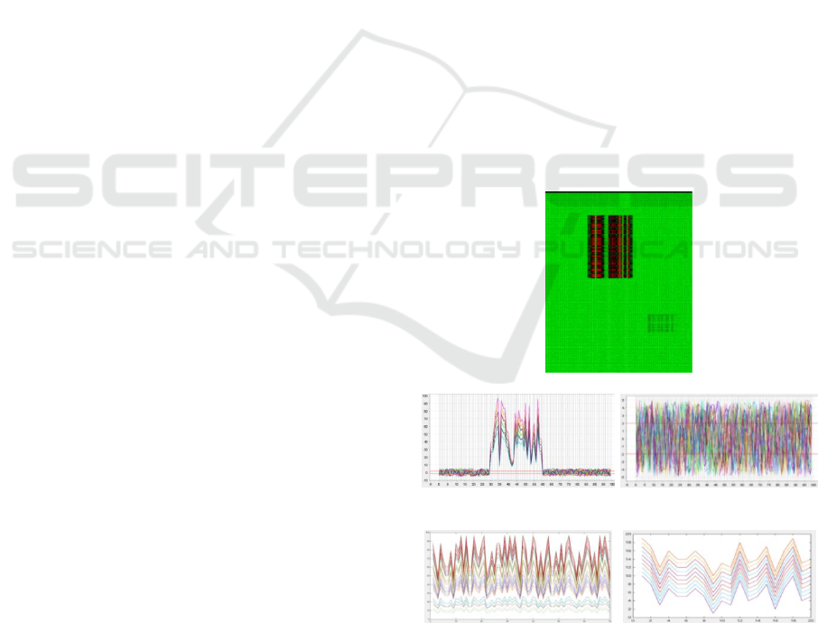
and biclustering is visualised in Figure 1. The

original dataset with 200 rows and 100 columns is

shown in Figure 1 (a) with two biclusters. Figure 1

(b, c) are the clusters by a clustering technique and

Figure 1 (d, e) are the detected biclusters by a

biclustering technique. Figure 1 (b, d), and Figure 1

(c, e) refer to a same set of samples with different

subset of features (Figure 1 (b, c) include all features

in the dataset). As it is clear, information that is

more valuable can be obtained from biclustering

technique (Figure 1 (d, e)). Biclustering has found

many applications in different fields e.g. disease

detection (Maulik et al., 2013); social networks

clustering (Shafiq et al., 2013) and gene expression

analysis (Ben-Dor et al., 2003; Cheng and Church,

2000; Divina and Aguilar, 2006; Gan et al., 2005;

Gan et al., 2008; Ihmels et al., 2004; Golchin and

Liew, 2017; Cheng et al. 2008).

(a)

(b)

(c)

(d)

(e)

Figure 1: The difference between a clustering method (b

and c) and a biclustering method (d and e). The x-axis is

the feature indices and the y-axis is the expression values;

the original dataset with 200 rows and 100 columns is

shown in (a) with two biclusters.

Golchin, M. and Liew, A.

Bicluster Detection by Hyperplane Projection and Evolutionary Optimization.

DOI: 10.5220/0006710000610068

In Proceedings of the 11th International Joint Conference on Biomedical Engineering Systems and Technologies (BIOSTEC 2018) - Volume 3: BIOINFORMATICS, pages 61-68

ISBN: 978-989-758-280-6

One way to detect biclusters with linear coherent

structure in datasets is via geometric biclustering. In

geometric biclustering, each bicluster is described

with a linear equation. In computer vision, an

effective way to detect linear structures in an image

is the Hough Transform (HT) (Hough, 1962). HT

identifies lines in the dataset by a voting procedure,

which is performed in Hough space. It maps the x-y

coordinates into ρ-θ parameter space where ρ is the

distance of the line to the origin and θ is the angle of

the normal vector. HT parametrizes pattern space

then projects all points into the parameter space,

from which the local maxima in an accumulator

space imply the line candidates. Gan et al. (2005,

2008) propose to detect a bundle of hyperplanes

representing biclusters within a dataset using HT

method. However, HT is computationally expensive

and the storage memory requirement is high. This

makes HT un-scalable for high dimensional data. In

order to overcome the large memory and

computational time, Zhao et al. (2008) proposed to

apply HT in column-pair space. In order to combine

the coherent sub-biclusters B

= (r

, c

) and B

= (r

, c

), they used the operation B

 B

= (r

∩ r

, c

 c

). Liu et al. (2014) and Wang et al. (2012) also

used the same method to combine column pair sub-

biclusters. Wang and Yan (2013) used a graph

spectrum algorithm to combine sub-biclusters. All

these efforts in using HT show the effectiveness of

HT in detecting biclusters. However, the heuristic

combination strategies may fail with regard to detect

and combine sub-biclusters to generate bigger

biclusters and may converge to local maxima.

In order to overcome the space usage and

complexity of Hough transform, evolutionary

algorithms and heuristic search are introduced to

biclustering. In evolutionary algorithms, the merit

functions are very important to obtain good results.

However, the objectives that are applicable in

biclustering are often in conflict with each other.

Therefore, the single objective merit function is not

very useful for this kind of problem. Instead, multi-

objective evolutionary algorithms (Błażej et al.

2017; Winterhalter et al. 2014) are desired.

In this paper, we propose a multi-objective

strength Pareto front evolutionary algorithm based

on SPEA2 (Zitzler et al., 2001) for biclustering. Our

method uses a new heuristic search based on sample

Pearson correlation coefficient. We present

experimental results showing that our algorithm can

detect biclusters with linear coherent patterns well

compared to many state-of-the-arts.

2 METHODOLOGY

We consider a dataset as an m × n matrix of real

numbers. Let R = {r

, r

, …, r

} represents the rows

in the dataset and C = {c

, c

, …, c

} represents the

columns in the dataset. A bicluster is a set of rows

and columns with elements e

that follow a certain

pattern, where i  {1 .. m} and j  {1 .. n}. For

linear coherent patterns, we consider biclusters that

satisfy a linear relationship given by c

= Ac

+ B,

where c

 C, A is the coefficient matrix and B is

the constant vector. Linear relationship has been

used extensively in pattern recognition and machine

learning (Bishop, 2006) and linear coherent patterns

cover many biclusters of interest in many

applications (Gan et al., 2005, Gan et al., 2008,

Liew, 2016).

The general steps of the proposed method are

summarized in Pseudocode 1. Each step of the

algorithm is explained in details in the remaining of

this paper.

Pseudocode 1: The proposed framework

For maximum number of biclusters

Generate initial populations

For maximum number of iterations

Apply heuristic search for

each individual

Calculate the fitness

function for each individual

Generate Pareto front

Apply crossover and mutation

Apply the k-means algorithm to

the Pareto front

2.1 Population

In our method, we have two populations, i.e. a

normal population and an archive population,

hereinafter referred as population and archive,

respectively.

We encode each bicluster as an individual with a

fixed size m + n bit string where one indicates that

the corresponding row or column belongs to the

bicluster and zero otherwise. Figure 2 illustrates an

encoded bicluster. This bicluster is generated from a

dataset with 8 rows and 6 columns. In this bicluster

row indices {2, 3, 5, 8} and column indices {1, 2, 6}

are selected.

BIOINFORMATICS 2018 - 9th International Conference on Bioinformatics Models, Methods and Algorithms

Figure 2: The presentation of biclusters as an individual.

All the individuals are kept in the population and

only the best non-dominated individuals are added to

the archive. This helps to keep the best individuals

for the next steps and make a good mating pool

including the best non-dominated and dominated

individuals.

The size of the archive is fixed, so if the number

of non-dominated individuals is bigger than the size

of the archive, only individuals with small fitness

value and non-duplicated individuals from the

previous archive and the present population are

added to the archive. On the other hand, if the

number of non-dominated individuals is smaller than

the archive size, then dominated individuals with

higher fitness value from the present population are

added to the archive.

2.2 Heuristic Search

Due to the nature of the evolutionary algorithms, the

probability of having unwanted rows and columns in

a bicluster is high. A greedy heuristic search is

designed to remove these uncorrelated columns and

rows and to add correlated columns and rows to the

bicluster. In order to find correlated rows and

columns, sample Pearson correlation coefficient

(SPCC) is used. SPCC measures the linear

dependence between two variables and it is

calculated as in Equation (1)





















































































(1)

The value of τ can be from -1 to 1 with -1 and 1

show highest correlation and 0 shows no correlation.

The steps of the proposed heuristic search are

summarized in Pseudocode 2.

Pseudocode 2: Heuristic search

For each individual:

// Rows deletion

For all rows in a bicluster do

Calculate τ between a random row

in the bicluster and the

remaining rowsin the bicluster

If τ ≤ α

then count = count + 1

If counter ≥ 2/3 × n

then remove r

// Columns deletion

For all columns in the bicluster do

Calculate τ between a random

column c

in the bicluster and the

remaining columns in the bicluster

If τ ≤ α

then counter = counter

+ 1

If counter ≥ 2/3 * n

then remove c

// Rows addition

For a number of selected rows from

the dataset excluding the bicluster

10:

Calculate τ between a random row

from the selected rows and the

rows in the bicluster

11:

If τ ≥ α

then counter = counter

+ 1

12:

If counter ≥ 2/3 * n

then add r

the bicluster

// Columns addition

13:

For a number of selected columns

from the dataset excluding the

bicluster do

14:

Calculate τ between a random

column c

from the selected

columns and the columns in the

bicluster

15:

If τ ≥ α

then counter = counter

+ 1

16:

If counter ≥ 2/3 * n

then remove c

In this algorithm, α

, α

, and α

are the

user-defined thresholds to control the rate of row

deletion, column deletion, row addition, and column

addition, respectively. These values are determined

experimentally and are set to 0.98 in our

experiments.

2.3 Fitness Function

Biclustering has been shown to be NP-Hard (Cheng

and Church, 2000). In order to overcome this

problem, EA based biclustering algorithms have

been proposed. Divina and Ruiz (2006) used EA to

find biclusters in gene expression data. In their

method, they used three objectives plus a penalty

value for their evolutionary search and they

combined these objectives additively in a merit

function. However, the objectives i.e. size,

coherence, and row variance are in conflict with

each other by nature. So, multi-objective

evolutionary algorithms are introduced to overcome

this problem (Maulik et al., 2009; Seridi et al., 2015;

Golchin and Liew, 2017).

In this paper, a strength Pareto front multi-

objective evolutionary algorithm is used. The

conflicting objectives in our algorithm include the

size of a bicluster (S

) which we try to maximize and

Bicluster Detection by Hyperplane Projection and Evolutionary Optimization

the coherence of the bicluster (e

) which we try to

minimize. These two objectives are in conflict since

maximizing the size would increase the incoherence

of the bicluster.

2.3.1 Bicluster Size

In order to calculate the size of a bicluster, rows and

columns are considered separately and they are

added together by a weighted sum as in Equation (2)





























(2)

where w

and w

are weights that are assigned to

rows and columns, respectively; m and n are the

number of rows and columns in the dataset; m

and

are the number of rows and columns in the

bicluster, respectively.

2.3.2 The Coherence of Patterns

In order to calculate the coherence of patterns, each

row in a data matrix is considered as a data point in

a high dimensional space where each column defines

a dimension and each element specifies a coordinate

value in the high dimensional space. The linear

pattern among the elements of the dataset makes a

hyperplane in the high dimensional space. In order

to find the hyperplane, the normal vector of the

hyperplane is computed. To do so, singular value

decomposition (SVD) is used. The SVD

decomposition of a matrix includes left singular

matrix U  R

m×m

, right singular matrix V  R

n×n

and

singular values S  R

m×n

in a way that



≥



≥ … ≥



≥ 0, r = min (m, n). The SVD of matrix M is

calculated as MV = US. According to Tomasi (2013)

the r

row of the left singular matrix represents the

normal vector of the hyperplane. The coherence of a

bicluster is calculated as how close the rows in a

bicluster are to the detected hyperplane. To find this

value, the root mean square error (RMSE) are

calculated by





































(3)

Here, r

is the number of rows in the bicluster, n

is the normal vector of the hyperplane, c is the

constant value of the hyperplane, p

represents each

row in the bicluster, ǁ•ǁ denotes the norm value of a

vector and • is the inner product of two vectors.

2.4 Pareto Front

In a single objective minimization problem, we try

to find min[f(x)] where f is a scalar fitness function,

x  S and S = {x  R

: h(x) = 0, g(x) ≥ 0} (objective

space). The multi-objective optimization problem is

denoted as min[f

(x), …, f

(x)], x  S and n > 1. In

multi-objective optimization, there is no unique

solution. Rather, there exists a set of solutions that

constitute the Pareto front solutions (Deb, 2014).

The Pareto front is defined by x*  S, if f

(x*) ≤ f

(x)

for all i  {1, …, n} (n is the number of objectives)

and at least one f

(x*) < f

(x). in this case, x*  S

dominates x  S (x*  x). x* is called a non-

dominated individual and x is called a dominated

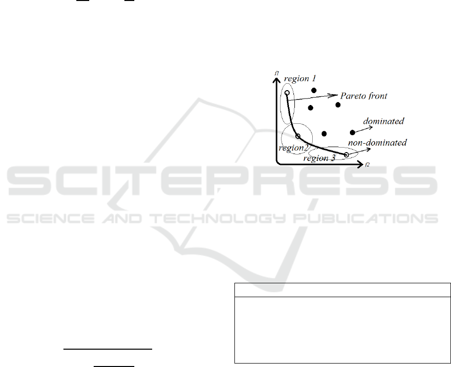
individual. These definitions are illustrated in Figure

Figure 3: The objective space with two objectives f

and f

;

hollow dots represent non-dominated individuals and

filled dots represent dominated individuals; Pareto front is

clustered using the k-means algorithm to detect the final

individual.

In order to constitute the Pareto front in the

proposed method, several values are calculated for

each individual.

Pseudocode 3: The Pareto front constitution

For each individual x in the

population p and the archive a do

S(x)=|{x* | x*  ap ˄ xx*}|

R(x)=





p ˄ x*



S(x*)

D(x)=1/(d

+ 2)

F(x)=R(x)+D(x)

S(x) is the strength value of each individual and

it shows the number of individuals it dominates. R(x)

is the raw fitness value and it is the sum of the

strength values of the individuals that dominates

individual x. Non-dominated individuals are not

dominated by any individuals, so their raw fitness

value should equal to zero. Density value D(x) is a

small value (< 1) to differentiate between the

individuals with similar raw fitness and it is

calculated as the inverse of Euclidean distance

between individual x and the k

individual. Finally,

BIOINFORMATICS 2018 - 9th International Conference on Bioinformatics Models, Methods and Algorithms

F(x) is the sum of raw fitness and density value and

it is the final value that is assigned to each

individual.

2.5 Crossover and Mutation

Single point crossover and bit string mutation are

applied to generate the next population. Rows and

columns undergo the crossover and mutation

separately.

The parents are selected based on binary

tournament selection by replacement from

individuals in the archive.

In crossover, a row or column index is randomly

selected. Then all the values in rows or columns

beyond that index are swapped between the two

parents. In mutation, a row or column index is

randomly selected and the value of that bit is

flipped.

2.6 Final Individual Selection

The last step of the proposed method is to find the

final individual among the Pareto front individuals.

The k-means algorithm is applied for this purpose.

The number of k is set to three in this study to

convert Pareto front to three separate regions and the

final individual is selected from region 2 as shown in

Figure 3. In this figure, f

denotes the size of the

bicluster and f

denotes RMSE.

3 RESULTS AND DISCUSSION

In order to qualify the performance of the proposed

method, we performed experiments on synthetic and

real gene expression datasets. We designed several

experiments with synthetic datasets to study

different aspects of the proposed algorithm. The

generated datasets include linear pattern biclusters

with different noise levels and different degree of

overlaps. In order to evaluate the performance of the

proposed algorithm, Jaccard index J is calculated for

each bicluster as in Equation (4):







































(4)

where r

and c

are the rows and columns of the

detected bicluster, respectively, r

and c

are the

rows and columns of the ground truth, and |•|

represents the number of elements.

Jaccard index calculates the ratio of similar rows

and columns over the total number of rows and

columns in the detected bicluster and the ground

truth. The value of Jaccard index differs from 0 to 1

where 1 indicates 100% similarity and 0 indicates no

similarity.

The proposed method is also compared with

several methods such as CC (Cheng and Church,

2000), xMotifs (Murali and Kasif, 2003), ISA

(Ihmels et al., 2004) and OPSM (Ben-Dor et al.,

2003). The results of CC, xMotifs, ISA and OPSM

are obtained using BicAT toolbox (Barkow et al.,

2006). The default parameters are used to generate

their results.

3.1 Synthetic Datasets

In the first experiment, the noise tolerance of the

proposed method in noisy datasets is considered.

The dataset consists of 50 rows and 50 columns with

a noisy background generated by a uniform

distribution U(-5,5). There are five hidden biclusters

in the dataset. The size of each bicluster is 10×10

and their values are generated randomly in a way

that the element values vary over the range from 6 to

30 and contain a linear pattern. Gaussian noise with

variance from zero to one degraded the biclusters.

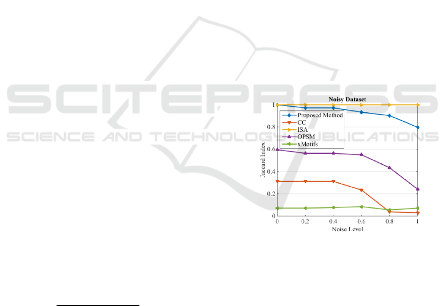
The results are visualized in Figure 4. The average

value of Jaccard index for all the detected biclusters

are used to plot the results.

Figure 4: Jaccard index of noisy dataset.

As it is clear ISA exhibits a robust behaviour

with respect to noise. The proposed method is still

relatively robust, but exhibited sensitivity and

dropped performance at higher noise levels. This is

caused by the use of sample Pearson correlation

coefficient, i.e. as the noise increases the tendency of

rows mismatch also increase. The xMotifs algorithm

performs the worst by detecting partially 2 biclusters

out of 5 biclusters. CC is able to detect only 3

biclusters which dropped to 2 when the noise level

increases. OPSM is able to detect all 5 biclusters

when the noise level is from 0 to 0.6 and it drops to

detect only 2 biclusters when the noise level is 0.8

Bicluster Detection by Hyperplane Projection and Evolutionary Optimization

and 1. The proposed method and ISA are able to

detect all five biclusters with different noise levels.

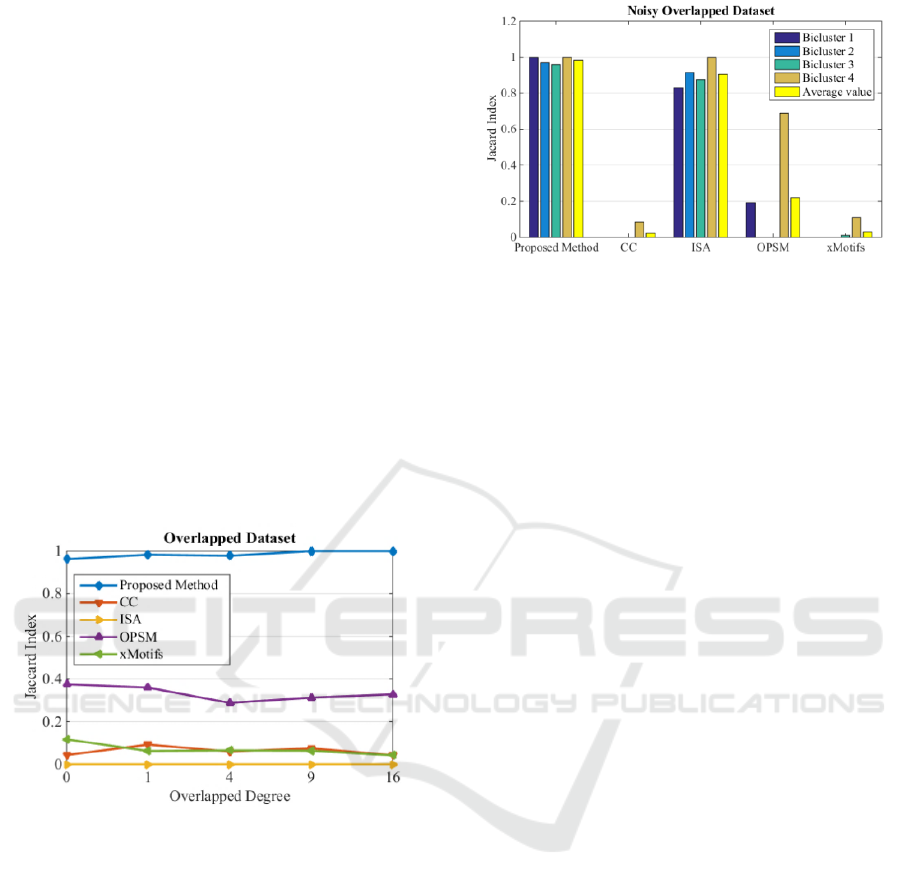
In the second experiment, the ability of the

algorithm in detecting overlapped biclusters is

studied. A dataset with the above property is

designed with 60 rows and 35 columns for the

background matrix with 2 biclusters of size 20×10

and 15×7. The results are visualized in Figure 5. The

average value of Jaccard index for the two biclusters

is used to plot the results. The y-axis shows the

overlapped degree, which is the number of

overlapped elements as in rows and columns e.g. 16

means 4 rows and 4 columns (4 degree).

In the noise level experiment, ISA performs very

poorly in this experiment and this algorithm is not

able to detect any bicluster at all. xMotifs and

OPSM are able to detect only one bicluster at any

overlapped degree. CC is able to detect only a few

rows and columns of both biclusters, as it is clear by

the value of its Jaccard index. The proposed method

out performed other methods in this experiment by

detecting almost 100% of all biclusters at different

overlapped degree.

Figure 5: Jaccard index of overlapped dataset.

The last experiment evaluates the performance of

the proposed method in detecting differing size of

biclusters in a dataset including both noisy and

overlapped biclusters. The background matrix

includes 200 rows and 60 columns with 4 biclusters.

The sizes of biclusters are 40×7, 25×10, 40×8 and

19×9. The biclusters are degraded by Gaussian noise

of variance 0.3 and the first two biclusters are

overlapped by degree of three (nine elements are

similar). The results are illustrated in Figure 6.

In this experiment, the proposed method

achieved the highest Jaccard index in all four

biclusters. The ISA algorithm is also able to detect

over 80% of the biclusters, especially when there is

no overlap in the biclusters.

Figure 6: Jaccard index of noisy overlapped dataset.

3.2 Real Dataset

Gene expression dataset is the expression level of

genes (rows) under several biological conditions

(columns). The purpose of biclustering is to discover

subgroups of genes, which are active in a subset of

conditions such that these groups show considerable

homogeneity from microarray data. In order to

assess the quality of detected biclusters in real

datasets, we performed an experiment on the yeast

Saccharomyces cerevisiae gene expression dataset

(Cho et al., 1998). The expression matrix of this data

set consists of 2884 genes (rows) and 17 conditions

(columns). In order to verify the functional

enrichment of detected genes in biclusters,

GenCodis (Tabas Madrid et al., 2012, Carmona Saez

et al., 2007, Nogales Cadenas et al., 2009) is used,

which has ten annotations for Saccharomyces

cerevisiae: GO Biological Process (BP); GO

Molecular Function (MF); GO Cellular Component

(CC); GOSlim Process (GP); GOSlim Function

(GF); GOSlim Component (GC); KEGG Pathways;

InterPro Motifs (IPM); Panther Pathways (PP); and

Transcription Factors (TF). From the 100 detected

biclusters, 100% achieved singular enrichment of

InterPro motifs, 95% achieved singular enrichment

of GOSlim Process, 93% achieved singular

enrichment of Panther Pathways, 80% achieved

singular enrichment of Go Biological Process, and

77% achieved singular enrichment of GO Cellular

Component. The remaining annotations had the

enrichment smaller than 10%. The graphical view of

co-occurrence annotation result for a detected

bicluster with 27 genes and 4 conditions is shown in

Figure 7.

BIOINFORMATICS 2018 - 9th International Conference on Bioinformatics Models, Methods and Algorithms

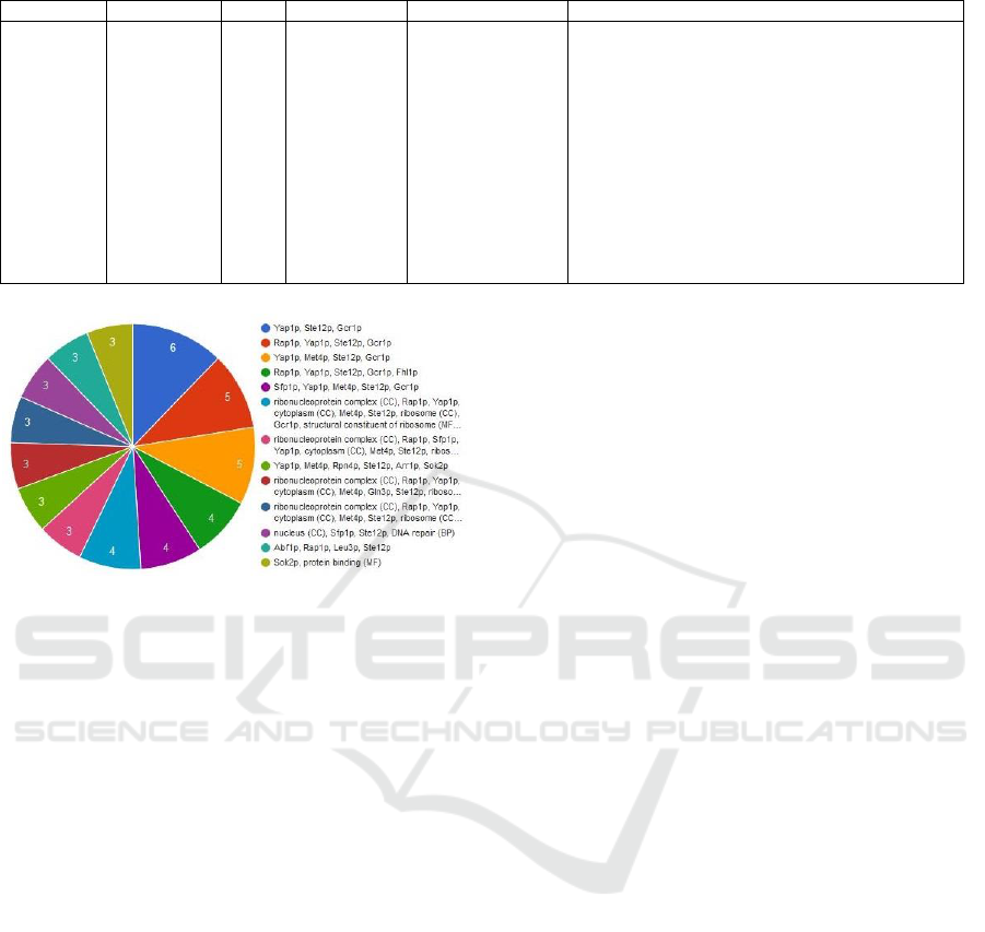
Table 1: Modular enrichment analysis of all annotations.

Genes

# Reference

# List

p-value

Corrected p-value

Annotations

YHL001W,

YDL081C,

YOL127W,

YKR094C

20 (7109)

4 (27)

6.54701e-07

4.97573e-05

GO:0030529: ribonucleoprotein complex (CC)

(Transcription factor) Rap1p

(Transcription factor) Yap1p

GO:0005737: cytoplasm (CC)

(Transcription factor) Met4p

(Transcription factor) Ste12p

GO:0005840: ribosome (CC)

(Transcription factor) Gcr1p

GO:0003735: structural constituent of ribosome (MF)

GO:0022625: cytosolic large ribosomal subunit (CC)

(KEGG) 03010: Ribosome

(Transcription factor) Ifh1p

GO:0002181: cytoplasmic translation (BP)

Figure 7: Number of genes per concurrent annotations.

Modular enrichment analysis (MEA) integrates

heterogeneous annotations from different sources,

which are BP, MF, CC, GP, GF, GC, KEGG, IPM,

PP, and TF, to find significant and enriched

combination of annotations in the list of detected

genes (Nogales Cadenas et al., 2009).

MEA of the smallest p-value for the same

bicluster as in Figure 8 is also presented in Table 1.

In this table, # reference shows the number of

annotated genes in the reference list. # list is the

number of annotated genes in the list of genes. From

27 detected genes in this bicluster, 4 genes have

modular enrichment of all annotations with a p-value

4.97573e-05. This indicates that the detected

bicluster is highly enriched.

4 CONCLUSIONS

In this paper, a new multi-objective evolutionary

based biclustering algorithm is introduced to

uncover hidden linear patterns in data. Our novel

contributions are as follows. First, our algorithm

takes advantage of the dimension information of the

hyperplane to reduce the time and space complexity

of the geometric biclustering. Secondly, our method

is able to detect different types of bicluster patterns

such as additive or multiplicative patterns without

pre-processing the dataset. Several synthetic

experiments are provided to validate the

performance of the algorithm. The results are also

compared with several well-known biclustering

methods, which show the superior performance of

the proposed method in different situations, i.e.,

noise and overlapping biclusters. Furthermore, a real

gene expression dataset is used to demonstrate the

accuracy of our method.

In the proposed method, only one bicluster is

detected at a time. For our future work, we want to

find multiple biclusters concurrently during the

optimization process.

ACKNOWLEDGEMENTS

Maryam Golchin is supported by the Australian

Government Research Training Program

Scholarship.

REFERENCES

Barkow, S., Bleuler, S., Prelić, A., Zimmermann, P. &

Zitzler, E. 2006. BicAT: A Biclustering Analysis

Toolbox. Bioinformatics, 22, 1282-1283.

Ben-Dor, A., Chor, B., Karp, R. & Yakhini, Z. 2003.

Discovering Local Structure in Gene Expression Data:

The Order-Preserving Submatrix Problem. Journal of

Computational Biology: A Journal of Computational

Molecular Cell Biology, 10, 373-384.

BISHOP, C. M. 2006. Pattern Recognition and Machine

Learning, New York, Springer.

Błażej, P., Mackiewicz, D., Grabińska, M., Wnętrzak, M.

& Mackiewicz, P. 2017. Optimization of Amino Acid

Replacement Costs by Mutational Pressure in

Bacterial Genomes. Scientific Reports, 7, 1061.

Carmona Saez, P., Chagoyen, M., Tirado, F., Carazo, J.

M. & Pascual Montano, A. 2007. GENECODIS: A

Web-Based Tool for Finding Significant Concurrent

Annotations in Gene Lists. Genome Biology, 8, R3.

Bicluster Detection by Hyperplane Projection and Evolutionary Optimization

Cheng, K.O., Law, N.F., Siu, W.C. & Liew, A. W. C.

2008. Identification of Coherent Patterns in Gene

Expression Data using an Efficient Biclustering

Algorithm and Parallel Coordinate Visualization.

BMC Bioinformatics, 9:210.

Cheng, Y. & Church, G. M. Biclustering of Expression

Data. Proceeding of Intelligent Systems for Molecular

Biology (ISMB), 2000. American Association for

Artificial Intelligence (AAAI), 93-103.

Cho, R. J., Campbell, M. J., Winzeler, E. A., Steinmetz,

L., Conway, A., Wodicka, L., Wolfsberg, T. G.,

Gabrielian, A. E., Landsman, D. & Lockhart, D. J.

1998. A Genome-Wide Transcriptional Analysis of the

Mitotic Cell Cycle. Molecular Cell, 2, 65-73.

Deb, K. 2014. Multi-Objective Optimization in Search

Methodologies. In: Burke, E. & Kendall, G. (eds.)

Search Methodologies. New York: Springer.

Divina, F. & Aguilar Ruiz, J. S. 2006. Biclustering of

Expression Data with Evolutionary Computation.

IEEE Transactions on Knowledge and Data

Engineering, 18, 590-602.

Gan, X. C., Liew, A. W. C. & Yan, H. Biclustering Gene

Expression Data Based on a High Dimensional

Geometric Method. Proceedings of 2005 International

Conference on Machine Learning and Cybernetics,

2005. IEEE, 3388-3393.

Gan, X. C., Liew, A. W. C. & Yan, H. 2008. Discovering

Biclusters in Gene Expression Data based on High-

Dimensional Linear Geometries. BMC Bioinformatics,

9:209.

Golchin, M. & Liew, A. W. C. 2017. Parallel Biclustering

Detection using Strength Pareto Front Evolutionary

Algorithm. Information Sciences, 415-416, 283-297.

Hough, P. V. 1962. Method and Means for Recognizing

Complex Patterns. United States patent application.

Ihmels, J., Bergmann, S. & Barkai, N. 2004. Defining

Transcription Modules using Large-Scale Gene

Expression Data. Bioinformatics, 20, 1993-2003.

Liew, A. W. C. 2016. Biclustering Analysis of Gene

Expression Data using Evolutionary Algorithms In:

IBA, H. & NOMAN, N. (eds.) Evolutionary

Computation in Gene Regulatory Network Research.

Hoboken, NJ, USA: John Wiley & Sons Inc.

Liu, B., Yu, C. W., Wang, D. Z., Cheung, R. C. & YAN,

H. 2014. Design Exploration of Geometric

Biclustering for Microarray Data Analysis in Data

Mining. IEEE Transaction on Parallel and Distributed

Systems, 25, 2540 - 2550.

Maulik, U., Mukhopadhyay, A. & Bandyopadhyay, S.

2009. Finding Multiple Coherent Biclusters in

Microarray Data using Variable String Length

Multiobjective Genetic Algorithm. IEEE Transactions

on Information Technology in Biomedicine, 13, 969-

975.

Maulik, U., Mukhopadhyay, A., Bhattacharyya, M.,

Kaderali, L., BRORS, B., Bandyopadhyay, S. & Eils,

R. 2013. Mining Quasi-Bicliques from HIV-1-Human

Protein Interaction Network: A Multiobjective

Biclustering Approach. IEEE/ACM Transactions on

Computational Biology and Bioinformatics, 10, 423-

435.

Murali, T. & Kasif, S. Extracting Conserved Gene

Expression Motifs from Gene Expression Data.

Proceedings of the Pacific Symposium on

Biocomputing, 2003. 77-88.

Nogales Cadenas, R., Carmona Saez, P., Vazquez, M.,

Vicente, C., Yang, X., Tirado, F., Carazo, J. M. &

Pascual Montano, A. 2009. GeneCodis: Interpreting

Gene Lists through Enrichment Analysis and

Integration of Diverse Biological Information. Nucleic

Acids Research, 37, W317-W322.

Seridi, K., Jourdan, L. & Talbi, E. G. 2015. Using

Multiobjective Optimization for Biclustering

Microarray Data. Applied Soft Computing, 33, 239-

249.

Shafiq, M. Z., Ilyas, M. U., Liu, A. X. & Radha, H. 2013.

Identifying Leaders and Followers in Online Social

Networks. IEEE Journal on Selected Areas in

Communications, 31, 618-628.

Tabas Madrid, D., Nogales Cadenas, R. & Pascual

Montano, A. 2012. GeneCodis3: A Non-Redundant

and Modular Enrichment Analysis Tool for Functional

Genomics. Nucleic Acids Research, 40, W478-W483.

Tomasi, C. 2013. Orthogonal Matrices and the Singular

Value Decomposition. Available:

https://www.cs.duke.edu/courses/fall13/compsci527/n

otes/svd.pdf [Accessed 17/01/2017].

Wang, D. Z. & Yan, H. 2013. A Graph Spectrum Based

Geometric Biclustering Algorithm. Journal of

Theoretical Biology, 317, 200-211.

Winterhalter, C., Nicolle, R., Louis, A., TO, C., Radvanyi,

F. & Elati, M. 2014. Pepper: Cytoscape App for

Protein Complex Expansion using Protein–protein

Interaction Networks. Bioinformatics, 30, 3419-3420.

Zhao, H., Liew, A. W. C., Xie, X. & Yan, H. 2008. A New

Geometric Biclustering Algorithm Based on the

Hough Transform for Analysis of Large-Scale

Microarray Data. Journal of Theoretical Biology, 251,

264-274.

Zitzler, E., Laumanns, M. & Thiele, L. SPEA2: Improving

the Strength Pareto Evolutionary Algorithm.

Proceedings of the Evolutionary Methods for Design,

Optimization and Control with Applications to

Industrial Problems (EUROGEN'01), 2001 Athens.

Greece. Eidgenössische Technische Hochschule

Zürich (ETH), Institut für Technische Informatik und

Kommunikationsnetze (TIK).

BIOINFORMATICS 2018 - 9th International Conference on Bioinformatics Models, Methods and Algorithms