
Fredholm Integral Equation for Finite Fresnel Transform
Tomohiro Aoyagi, Kouichi Ohtsubo and Nobuo Aoyagi
Faculty of Information Sciences and Arts, Toyo University, 2100 Kujirai, Saitama, 350-8585, Japan
Keywords: Fresnel Transform, Integral Equation, Eigenvalue Problem, Jacobi Method.
Abstract: The fundamental formula in an optical system is Rayleigh diffraction integral. In practice, we deal with
Fresnel diffraction integral as approximate diffraction formula. We seek the function that its total power is
maximized in finite Fresnel transform plane, on condition that an input signal is zero outside the bounded
region. This problem is a variational one with an accessory condition. This leads to the eigenvalue problems
of Fredholm integral equation of the first kind. The kernel of the integral equation is Hermitian conjugate and
positive definite. Therefore, eigenvalues are nonnegative and real number. By discretizing the kernel, the
problem depends on the eigenvalue problem of Hermitian conjugate matrix in finite dimensional vector space.
By using the Jacobi method, we compute the eigenvalues and eigenvectors of the matrix. We applied it to the
problem of approximating a function and evaluated the error.
1 INTRODUCTION
The integral theorem of Helmholts and Kirchhoff
plays an important role in the development of the
scalar theory of diffraction (Goodman, 2005).
Although scalar wave propagation is fully described
by a single scalar wave equation, fundamental
formula in an optical system is Rayleigh diffraction
integral. In practice, we deal with Fresnel diffraction
integral as approximate diffraction formula. The
Fresnel transform has been studied mathematically
and revealed the topological properties in Hilbert
space (Aoyagi, 1973). In recently, it is also used in
image processing, optical information processing,
optical waveguides and computer-generated
holograms. The extension of optical fields through on
optical instrument is practically limited to some finite
area. This leads to the spatially band-limited problem.
The effect of band limitation has been studied for an
optical Fourier transform, namely in the region of the
Fraunhofer diffraction. Up to now, sampling theorem
have been derived from band-limited effect in Fourier
transform plane and applied to application areas.
Moreover, sampling function system are orthonormal
system in Hilbert space. An orthonormal function
system may be considered as coordinate system in
some functional space.
In sampling theorem, it is important to develop the
orthogonal functional systems (Ogawa, 2009). It has
been also revealed the function to minimize the norm
of error on condition that
-norm of a function in
finite Fourier plane is not exceeding a constant (Kida,
1994). In the literature, there are many examples of
band-limited function in the Fourier transform, its
applications and reference therein (Jerri, 1977).
However, the band-limited effect in Fresnel transform
plane is not revealed sufficiently.
In this paper, we seek the function that its total
power is maximized in finite Fresnel transform plane,
on condition that an input signal is zero outside the
bounded region. This problem is a variational one
with an accessory condition. This leads to the
eigenvalue problems of Fredholm integral equation of
the first kind. The kernel of the integral equation is
Hermitian conjugate and positive definite. Therefore,
eigenvalues are real non-negative numbers. By
discretizing the kernel and using the value of the
representative points, the problem depends on the
eigenvalue problem of Hermitian conjugate matrix in
finite dimensional vector space. By using the Jacobi
method, we compute the eigenvalues and
eigenvectors of the matrix. In general finite
dimensional vector spaces (
), the eigenvalues of
Hermitian matrix are real numbers and then
eigenvectors from different eigenspaces are
orthogonal. We consider the application of the
eigenvectors to the problem of approximating a
function and evaluate the error between original test
functions and approximating functions.
286
Aoyagi, T., Ohtsubo, K. and Aoyagi, N.
Fredholm Integral Equation for Finite Fresnel Transform.
DOI: 10.5220/0006709202860291
In Proceedings of the 6th International Conference on Photonics, Optics and Laser Technology (PHOTOPTICS 2018), pages 286-291
ISBN: 978-989-758-286-8
Copyright © 2018 by SCITEPRESS – Science and Technology Publications, Lda. All rights reserved

2 FRESNEL TRANSFORM
Assume that we place a diffracting screen on the
plane. The parameter represents the normal
distance from the input plane. Let , be the
coordinates of any point in that plane. Parallel to the
screen at is a plane of observation. Let , be the
coordinates of any point in this latter plane. If
represents the amplitude transmittance, then the
Fresnel transform is defined by
exp
exp
where is the wave number and
. The
inverse Fresnel transform is defined by
exp
exp
Figure 1 shows a general optical system and its
coordinate system. Fresnel transform is a bounded,
linear, additive and unitary operator in Hilbert space.
3 EIGENVALUE PROBLEM
To simplify the discussion, we consider only one-
dimensional Fresnel transform. The one-dimensional
Fresnel transform is defined by
×exp
where we set the wave number unit. The inverse
Fresnel transform is defined by
Figure 1: Sketch of a general optical system.
×exp
Assume that
is limited within the finite region
on the -plane and its total power
, namely the
inner product of the function, is constant.
where
denotes the complex conjugate function
of
. Assume that
is the Fresnel transform of
the function
which is bounded by a finite region
, that is,
Then, the total power
of
in the bounded
region is
exp
where the kernel function
is defined by
We seek the function
that maximizes
provided that the total power
is fixed. This
problem is a variational one with an accessory
condition. We use the method of Lagrange multiplier
to solve this problem.
Let us define two functions,
and
as
followings.
Fredholm Integral Equation for Finite Fresnel Transform
287

We want to maximize the function
, subject to
the constraint
. Setting the Lagrange multiplier,
Lagrangian functional is defined by
We set the gradient of Lagrangian to zero, that is,
where indicate the gradient.
By Eq. (7) and Eq. (9), we obtain
We conclude that
This is the Fredholm integral equations of the first
kind. This equation corresponds to some modification
of the integral equation for prolate spheroidal wave
functions (Slepian and Pollak, 1961).
According to Eq. (7), we can write
Therefore, the kernel
of the integral
equation is positive definite.
To prove the eigenvalues of above integral equation
are nonnegative, it is necessary to show
.
In this case is an eigenvalue, is an eigenvector
and
indicates the norm in Hilbert space (Yosida,
1980). Therefore, by replacing
with
and
taking Eq. (14) into consideration, we can write
Figure 2: Absolute values of the kernel of the integral
equation. Variable ‘a’ is the non-zero region on Fresnel
transform plane, i.e. |x|≤a.
Therefore, the eigenvalues of the integral equation are
nonnegative and real number.
Let us consider the kernel of the integral equation.
If object plane and Fresnel transform plane are
bounded by finite regions, the kernels of the integral
equation are calculated analytically as the kernel
function. We set the finite region in Fresnel
transform plane .
Figure 2 shows the absolute value of the kernel in Eq.
(17). In this case we set .
Let us consider the complex conjugate of the kernel
of the integral equation.
Therefore, the kernel is of Hermitian symmetry.
4 COMPUTER CALCULATION
4.1 Eigenvalues and Eigenvectors
It is difficult in general to seek the strict solution of
the integral equation. So we desire to seek the
approximate solution in practical exact accuracy
(Kondo, 1954). By discretizing the kernel function
and using the value of the representative points, we
can write
PHOTOPTICS 2018 - 6th International Conference on Photonics, Optics and Laser Technology
288
where , are the natural number, . The
matrix
is the Hermitian matrix if the kernel is
discretized evenly-spaced and . Therefore, the
eigenvalue problems of the integral equation depend
on a one of the Hermitian matrix in finite dimensional
vector space. However, although the diagonal
elements of the matrix are indeterminate form, we
seek the limit value. If
, we can write
We can replace
with .
In general finite dimensional vector spaces (
), the
eigenvalues of Hermitian matrix are real numbers and
then eigenvectors from different eigenspaces are
orthogonal (Anton and Busby, 2003).
We use the Jacobi method to compute eigenvalues
and eigenvectors of the matrix (Press et al., 1992).
Jacobi method is a procedure for the diagonalization
of complex symmetric matrices, using a sequence of
plane rotations through complex angles (Seaton,
1969). It works by performing a sequence of
orthogonal similarity updates
with the
property that each new is more diagonal than its
predecessor. In this update is an orthogonal matrix.
Eventually, the off-diagonal elements are small
enough to be declared zero (Golub and Van Loan,
1996). Finally, it can calculate all eigenvalues and
eigenvectors.
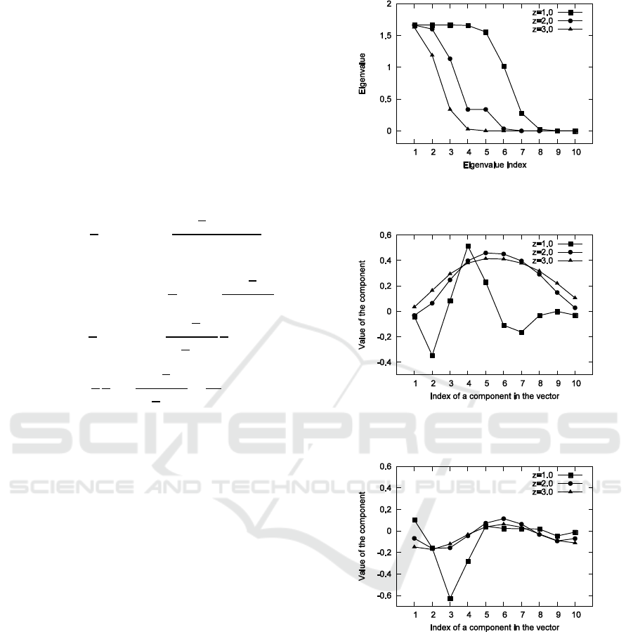
Figure 3 shows the eigenvalues in descending order,
if z is 1.0, 2.0 and 3.0. They are nonnegative and real
number. Figure 4 shows the real part of the
eigenvectors for the largest eigenvalue. Because of 10
dimensional vector space, except for this, there are 9
eigenvectors. Figure 5 shows the imaginary part of
the eigenvectors for the largest eigenvalue. In this
case, the finite region S in Fresnel transform is
. Its vector space is spanned by these eigenvectors.
Figure 3: Plots of the eigenvalues in descending order.
a=3.0.
Figure 4: Plots of the eigenvectors for the largest eigenvalue.
Its real part. a=3.0.
Figure 5: Plots of the eigenvectors for the largest eigenvalue.
Its imaginary part. a=3.0.
4.2 Evaluation of Functions
We consider the application of the above eigenvectors
to the problem of approximating a function.
Theoretically, we deal with a problem of expressing
an arbitrary element on a finite -dimensional
Hilbert space
with an orthonormal basis.
In
, every element can be expressed as a linear
combination of orthonormal basis (Reed and Simon,
1972). For any element in
, by using
orthonormal basis
, we can write
Fredholm Integral Equation for Finite Fresnel Transform
289

and
where indicates an identity operator and
is a
bracket.
Now, we set . Let us consider the set
of
all 10-tuples
where
are complex numbers.
Figure 6 shows the original test vector in
, which
real part is (0, 0, 1, 1, 1, 1, 1, 1, 0, 0) and imaginary
part is all zero. Figure 7 shows another original test
vector in
, which real part is (0, 0, 0.5, 1, 0.5, -0.5,
-1, -0.5, 0, 0) and imaginary part is all zero. Figure 8
shows third original test vector in
, which real part
is (0, 0, 0.5, 1, 0.5, -0.5, -1, -0.5, 0, 0) and imaginary
part is (0, -0.5, -0.5, -0.5, 0, 0, 0.5, 0.5, 0.5, 0). The
eigenvectors which are calculated by the Jacobi
method are automatically orthonormal. So, by using
Eq. (23), we have evaluated the error between the
original test vector and the approximating vectors
which are consisted of the eigenvectors. Figure 9
illustrates the mean square error versus the number of
eigenvectors. The mean square error is defined by
where
is the sum in Eq. (23) up to , is the
original vector, and
is the
-norm. From Fig. 9,
we can see that the error decreases with increasing
number of eigenvectors used in the expansion. The
problem of time consuming arises with increasing
vector dimension.
Figure 6: Example 1: Plots of the real parts of the original
test vector.
Figure 7: Example 2: Plots of the real parts of the original
test vector.
Figure 8: Example 3: Plots of the original test vector. Filled
squares indicate the imaginary part.
Figure 9: Plots of the normalized mean square error versus
the number of eigenvectors.
5 CONCLUSIONS
We have sought the function that its total power is
maximized in finite Fresnel transform plane, on
condition that an input signal is zero outside the
bounded region. We have showed that this leads to
the eigenvalue problems of Fredholm integral
equation of the first kind. By discretizing the kernel
and using the value of the representative points, the
problem depends on the eigenvalue problem of
Hermitian conjugate matrix in finite dimensional
PHOTOPTICS 2018 - 6th International Conference on Photonics, Optics and Laser Technology
290

vector space. By using the Jacobi method, we
compute the eigenvalues and eigenvectors of the
matrix. Furthermore, we applied it to the problem of
approximating a function and evaluated the error. We
confirmed the validity of the eigenvectors for the
Fresnel transform by computer simulations. In this
study, there are many parameters, especially, band-
limited area , , and . It is necessary to consist of
orthogonal functional systems with the optimal
parameters for finite Fresnel transform in application
of an optical system. In our Hermitian matrix, its
elements depend on the parameter . It is
necessary to reveal the property of the matrix with
such parameter and its effect of the eigenvalues and
the eigenvectors. Moreover, in general, the matrix
given by discretizing the kernel of the integral
equation is not the Hermitian matrix. If so, it is
difficult to compute accurately all eigenvalues and
eigenvectors. It is also necessary to consider other
computational methods for this. These become the
future problems. In our further problem, theoretically,
it is important to search for a spectral representation
of finite Fresnel transform in Hilbert space.
REFERENCES
Aoyagi, N., 1973. Theoretical study of optical Fresnel
transformations. Dr. Thesis, Tokyo Institute of
Technology, Tokyo.
Goodman, J., 2005. Introduction to Fourier optics. Roberts
& Company Publishers, Colorado, 3
rd
edition.
Ogawa, H., 2009. What can we see behind sampling
theorems? IEICE Trans. Fundam. E92-A, 688-695.
Kida, T., 1994. On restoration and approximation of multi-
dimentional signals using sample values of transformed
signals. IEICE Trans. Fundam. E-77-A, 1095-1116.
Jerri, A., 1977. The Shannon sampling theorem –its various
extensions and applications: a tutorial review. Proc.
IEEE, Vol. 65, No. 11, 1565-1596.
Slepian, D., Pollak, H., 1961. Prolate spheroidal wave
Functions, Fourier analysis and uncertainty -I. Bell
Syst. Tech. J. 40, 43-63.
Yosida, K., 1980. Functional Analysis, Springer-Verlag,
Berlin, 6
th
edition.
Kondo, J., 1954. Integral equation, Baifukan.
Tokyo[Japanese].
Press, W., Teukolsky, S., Vetterling, W., Flanney, B., 1992.
Numerical recipes in C, Cambridge University Press.
Cambridge, 2
nd
edition.
Anton, H., Busby, R., 2003. Contemporary linear algebra,
John Wiley & Sons, Inc., NJ.
Reed, M., Simon, B., 1972. Methods of modern
mathematical physics, Vol. 1, Academic Press, New
York.
Seaton, J., 1969. Diagonalization of complex symmetric
matrices using a modified jacobi method. Comp. J. 12,
156-157.
Golub, G., Van Loan, C., 1996. Matrix computations. Johns
Hopkins University Press, Maryland, 3
rd
edition.
Fredholm Integral Equation for Finite Fresnel Transform
291
