CRVM: Circular Random Variable-based Matcher
A Novel Hashing Method for Fast NN Search in High-dimensional Spaces
Faraj Alhwarin, Alexander Ferrein and Ingrid Scholl
Mobile Autonomous Systems & Cognitive Robotics Institute, FH Aachen University of Applied Sciences, Aachen, Germany
Keywords:
Feature Matching, Hash Tree, Fast NN Search.
Abstract:
Nearest Neighbour (NN) search is an essential and important problem in many areas, including multimedia
databases, data mining and computer vision. For low-dimensional spaces a variety of tree-based NN search
algorithms efficiently cope with finding the NN, for high-dimensional spaces, however, these methods are in-
efficient. Even for Locality Sensitive Hashing (LSH) methods which solve the task approximately by grouping
sample points that are nearby in the search space into buckets, it is difficult to find the right parameters. In
this paper, we propose a novel hashing method that ensures a high probability of NNs being located in the
same hash buckets and a balanced distribution of data across all the buckets. The proposed method is based on
computing a selected number of pairwise uncorrelated and uniformly-distributed Circular Random Variables
(CRVs) from the sample points. The method has been tested on a large dataset of SIFT features and was
compared to LSH and the Fast Library for Approximated NN search (FLANN) matcher with linear search
as the base line. The experimental results show that our method significantly reduces the search query time
while preserving the search quality, in particular for dynamic databases and small databases whose size does
not exceed 200k points.
1 INTRODUCTION
The Nearest Neighbour (NN) search is one of the
most basic and time-consuming processes in many
applications such as machine learning, multimedia
databases, data mining, computer vision and image
processing. In many of these applications, the data
are typically represented as high-dimensional vec-
tors. For example, a local feature extraction operation
on an image will result in hundreds of dimensions.
Consider a database of points P ⊂ R
d
are given as
P =
{
p
1
, p
2
, p
3
,. . . , p
n
}
. Now, the problem of NN
search is to find the closest point in P to a given query
point q using some similarity measure (e.g., the Ham-
ming or Euclidean distance).
NN(P,q) = {p ∈ P | ∀p
i
∈ P ∧ p
i
6= p
: dist(p,q) 6 dist(p
i
,q)}
The simplest solution for this problem is scanning
the whole database, computing the distances from the
query point to every point in the database sequen-
tially yielding the point with the smallest distance.
However, the running time of this operation is pro-
portional to the number and dimensionality of data
points. Therefore, this solution becomes dramati-
cally inefficient for high-dimensional and large-scale
databases (Har-Peled et al., 2012).
Over the last three decades, a lot of research
has addressed the problem of finding efficient solu-
tions for the NN search problem in high-dimensional
spaces. The proposed solutions have in common that
they organise the database contents in complex data
structures (trees, graphs or hash tables) in such a way
that querying a NN can be found without exploring
the whole database. Unfortunately, the operation of
storing new data into data structure as well as query-
ing the data structure keeps growing exponentially in
the number of dimensions. Recently, many papers
have been published to overcome this problem by ap-
proximating the search for NN; instead of reporting
the closest point to the query, it is allowed to report
any point within a distance less than (1 + ε) times the
distance between the query and its exact NN. The Ap-
proximated NN search (ANN) is sufficient for some
applications and search can be performed in polyno-
mial time w.r.t. the data dimensionality.
In this paper, a novel hashing method for the NN
search in high-dimensional space is proposed. Our
method is based on extracting several uncorrelated
and uniformly-distributed Circular Random Variables
(CRVs) from the data to be searched. These CRVs
214
Alhwarin, F., Ferrein, A. and Scholl, I.
CRVM: Circular Random Variable-based Matcher - A Novel Hashing Method for Fast NN Search in High-dimensional Spaces.
DOI: 10.5220/0006692802140221
In Proceedings of the 7th International Conference on Pattern Recognition Applications and Methods (ICPRAM 2018), pages 214-221
ISBN: 978-989-758-276-9
Copyright © 2018 by SCITEPRESS – Science and Technology Publications, Lda. All rights reserved

are then used to cluster the nearby data in the search
space into sub-spaces. Seeking the NN of some query
then means that only the corresponding sub-space has
to be explored instead of the whole search space. This
leads to a significant lower query time.
The remainder of the paper is organised as fol-
lows. In the next section, we review the related work
that has addressed the problem of NN search in high-
dimensional spaces. In Section 3, we introduce our
method based on CRVs and show its application for
SIFT features in Section 4. In Section 5, we evaluate
our method on a number of datasets of SIFT features
(with different sizes) and compare it with the LSH and
FLANN matcher. Finally we conclude the paper in
Section 6.
2 RELATED WORK
The simplest way to find the NN is a brute-force
search which includes computing all the metric dis-
tances from a query point to every point in the dataset
for finding the point with the smallest distance. This
algorithm finds the exact NN, but it is inefficient for
large datasets and high-dimensional spaces. The NN
search can be accelerated by relaxing the problem and
searching for the Approximated NN (ANN) instead
of the exact one. In general, ANN search algorithms
can be divided into three major categories: graph-
based, tree-based, and hash-based algorithms (Muja
and Lowe, 2009).
The graph-based algorithms construct a graph of
nodes and edges where the nodes represent the data
points and the edges connect each two neighbouring
points; edge weights reflect how close two points are
in the dataset. In the literature, many strategies to ex-
plore graphs have been published. In (Hajebi et al.,
2011), the starting points are chosen randomly and
a hill-climbing strategy is used. Another approach
is shown in (Sebastian and Kimia, 2002). There, a
few well-separated nodes are used as starting points
and the graph is then explored in a best-first order.
However, the graph-based algorithms suffer from the
high computational cost for the construction of the
NN graph structure. In spite of this, tree-based algo-
rithms are founded on the recursive partitioning of the
search space into sub-spaces. The most widely used
algorithm in this class is the k-d tree (Bentley, 1975;
Friedman et al., 1977). The k-d tree is a k-dimensional
binary tree which partitions the space hierarchically
resulting in a tree-based data structure. To search for
the NN, the k split coordinates of the query point are
used to determine the NN leaf node. Then, the lin-
ear search is performed to determine the closest point
within the NN leaf. The k-d tree operates successfully
in low-dimensional search space, but the performance
degrades exponentially with an increasing number of
dimensions. To overcome this restriction, many vari-
ations of the k-d tree approach were introduced by re-
laxing the NN search (Beis and Lowe, 1997; Arya
et al., 1998). Silpa-Anan et al. (Silpa-Anan and Hart-
ley, 2008) proposed the use of multiple randomised
k-d trees, which are created by choosing the split di-
mensions randomly from among a few dimensions
for which the data have a high variance. A constant
number of trees are built using independent random
choices. While searching for a query point, a single
priority queue is maintained across all the randomised
trees so that the search results can be ordered by the
increasing distance to each bin boundary. Another ex-
ample of a tree-based algorithms is the hierarchical
k-means tree (Fukunaga and Narendra, 1975). The
hierarchical k-means tree partitions the space hierar-
chically by using the k-means clustering algorithm in-
stead of using hyper-planes as in the case of the k-d
trees and its variants. The k-means clustering algo-
rithm determines a set of k points randomly (called
centroids). Then, k initial clusters are created by as-
sociating every data point with the nearest centroid.
The centroids are updated at each iteration by setting
them to the cluster means. This procedure is repeated
until convergence is achieved.
The most popular hash-based method for ANN
search is the Locality-Sensitive Hashing(LSH). The
LSH scheme was proposed by Indyk et al. (Indyk and
Motwani, 1998) for use in binary Hamming space and
was later extended by Datar et al. (Datar et al., 2004)
for the use in Euclidean space. The primary choice
of constructing an LSH function for the Euclidean
space is to project data points (represented as vectors
in R
d
) along a randomly chosen line (identified by a
random vector) which is segmented into intervals of
the same width. Then, data points projected to the
same interval are viewed as colliding in the hashing
scheme and each interval is considered as a bucket.
In (Andoni and Indyk, 2008), Andoni and Indyk used
a set of hash functions to cluster data points that are
nearby in the search space into the same bucket with
high probabilities. The performance of hash-based
algorithms highly relies on the quality of the hash
functions used and the tuning of algorithmic param-
eters. Therefore, many papers addressing these issues
have been published (e.g. (Kulis and Grauman, 2009;
Wang et al., 2010; Bawa et al., 2005)). In (Muja and
Lowe, 2009), Muja and Lowe compared many dif-
ferent algorithms for ANN search using datasets with
a wide range of dimensionality; they found that two
algorithms obtained the best performance, depending
CRVM: Circular Random Variable-based Matcher - A Novel Hashing Method for Fast NN Search in High-dimensional Spaces
215

on the dataset and the desired precision. These al-
gorithms used either the hierarchical k-means tree or
the multiple randomised k-d trees. They developed
a Fast Library for ANN search (FLANN) in high di-
mensional spaces. FLANN contains a collection of
the best algorithms for NN search and an automatic
mechanism for choosing the best algorithm and opti-
mal parameters depending on the dataset.
In this paper, we will introduce a novel hashing
method for NN search for high dimensional spaces.
The idea is to extract a set of CRVs from the dataset,
so that they are pairwise uncorrelated and tend to be
uniformly-distributed. The CRVs are then used to
hash the dataset points into one or few hash-trees.
For each set of pairwise uncorrelated and uniformly-
distributed CRVs, a hash tree can be constructed. De-
spite the simplicity of our method, it outperforms all
the state-of-the art methods for ANN search in high-
dimensional spaces specially for dynamic databases;
it does not require a complex data structure, training
phase, or parameter tuning operation.
3 CRV-BASED MATCHING
In this section, we outline the CRV-based matching al-
gorithm. We start with defining the Circular Random
Variables (CRVs).
Definition 1. Let x = (x
0
.. . x
n−1
)
T
be a n-
dimensional descriptor vector. We divide x into k
segments s
0
,. . . , s
k−1
, each of length l with k = d
n
l
e.
Each segment s
i
contains the following descriptor
components s
i
= {x
i·l
,x
i·l+1
,. . . , x
i·l+(l−1)
}. We asso-
ciate to each segment the index of the maximum value
as a random variable v
i
with v
i
= { j ∈ [0, l − 1] |
x
i·l+ j
is the maximum value in s
i
}.
Once the random variables v
i
are calculated for
all segments, a hash tree with l
k
leaves can be con-
structed, where the hash keys are determined by a
polynomial of order (k − 1) according to
h(x) = I =
k−1
∑
i=0
l
i
· v
i
. (1)
l denotes the CRV period and k the number of the
uncorrelated and uniformly-distributed CRVs that can
be extracted from the descriptor vector.
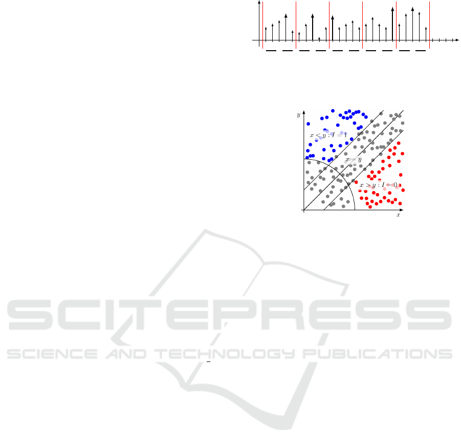
For an example illustrated in Fig. 1, the data points
are segmented with a period l = 5, each segment s
i
gets a value v
i
equal to the index of peak value in the
respective segment.
Becaue neibouring points have similar descrip-
tors, the CRVs computed from these descriptors tend
to be identical, which lead to hash neibouring points
into the same hash-tree leaf with high probability.
v
i
l = 5
x
0
x
5
x
10
x
15
x
20
x
25
| {z }
S
0
|
{z }
S
1
|
{z }
S
2
|
{z }
S
3
|
{z }
S
4
v
0
= 3 v
1
= 2 v
2
= 0 v
3
= 4 v
4
= 2
. . .
Figure 1: The extraction of CRVs from a data point repre-
sented as d-dimensional vector. In this example, the CRV
period is 5.
Figure 2: 2D classification results using one CRV v.
For the sake of simplicity, our idea is illustrated
in Fig. 2 for two-dimensional search space. For this
case, the whole vector is considered as one segment.
Therefore the period of the random variables is l = 2
and only one CRV v can be extracted. If the ab-
scissa of a feature is larger than the ordinate (x > y)
we get v = 0 (red features in Fig. 2, otherwise y > x
yields v = 1 (blue dots in the figure). For boundary
points, that at least one of whose segments has no
dominate maximum (grey dots in Fig. 2), we get a
boundary problem. In this case, boundary problem
can be avoided by adding boundary points to both
hash leaves.
In the general case (l > 2 and k > 1), the boundary
problem is solved by considering not only the maxi-
mum indices that define the CRVs, but also the second
maximum indices during determining the hash keys
of boundary points, when the second to first maxi-
mum ratio greater than a certain threshold T . This ra-
tio threshold can be used to make trade-off between
search speed and accuracy. This consideration can
be taken into account while storing or/and querying
stages. To explain this, we assume that we have a
dataset of 6D points, so we can segment each point
vector into two segments of length 3. The dataset
points will be stored in a hash tree of 9 leaves as
shown in Fig. 3.
While querying, if both segments of the query
point have dominate maxima (as the case of point
A in table 1), then only one of the 9 leaves have to
be searched. If one of the segments has no dominate
maxima (as the case of points B and C), then we
have to consider the maximum and the second maxi-
mum and hence two leaves have to be searched. In
ICPRAM 2018 - 7th International Conference on Pattern Recognition Applications and Methods
216

root
v
0
= 0
v
1
= 0
...
v
1
= 1
A, D, ..
v
1
= 2
D, ..
v
0
= 1
v
1
= 0
B, ..
v
1
= 1
...
v
1
= 2
...
v
0
= 2
v
1
= 0
B, C, ..
v
1
= 1
C, D, ..
v
1
= 2
D, ..
Figure 3: Hash tree for 6D dataset with two CRVs of pe-
riod=3.
the worst case that both segments have no dominate
maxima (as in the case of point D), then we need to
explore 4 leaves out of 9. For better explanation, table
1 shows the maximum, second maximum and their in-
dices of two segments for 4 example points, and Fig.
3 shows how they are stored( or queried )in the hash
tree, when the ratio threshold T is set to 0.5.
One property of the above hash function is that
features are mapped uniformly over the integer in-
dices of Eq. 1 if (1) the used CRVs are uniformly-
distributed; and (2) the CRVs are pairwise uncorre-
lated.
To examine whether the CRVs meet the
uniformly-distributedness condition, their proba-
bility density functions (PDF) are estimated from
a large dataset of points. The PDFs are computed
by building histograms of the CRV values ranging
between [0, l − 1]. Once the PDFs are constructed, the
χ
2
test is used to quantitatively evaluate the goodness
fit to the uniform distribution.
To examine, whether the CRVs meet the pairwise
uncorrelatedness condition, it is necessary to measure
the dependence between each pair of them. The most
familiar measure of dependence between two quanti-
ties is the Pearson product-moment correlation coeffi-
cient. For CRVs, the Circular Correlation Coefficient
(CCC) is used to measure the association between two
circular variables.
Once the CCC and the test statistic values are
computed for all the extracted CRVs, a subset of them
is chosen so that CCC and x values are as small as
possible. An example with CCCs computed for SIFT
features is shown in Figure 4. Based on the CCC, only
uncorrelated CRVs are chosen to construct a hash tree
and to hash dataset points into it. When querying a
query point, its hash key is determined and the NN
search is restricted only to points having the same
hash key.
The above conditions ensure that the data are
evenly distributed over all the buckets. This leads to
the following observation.
Table 1: Maximum, second maximum and corresponding
indices of 4 6D points.
point
v
1
v
2
1max-Id 2max-Id 1max-Id 2max-Id
A 100- 0 40-1 120-1 50-2
B 130-1 110-2 100-0 10-2
C 60-2 5-1 20-1 18-0
D 80- 0 79-2 60-2 59-1
Corollary 1. For a database of size S, and a num-
ber of buckets b = l
k
, we can calculate the size of ev-
ery bucket as B =
S
b
. Therefore, compared to linear
search, the query process can theoretically be sped
up by a factor ranging from f = (
l
2
)
k
(if all segments
do not have dominate maxima) to f =
S
B
= l
k
(if all
segments have dominate maxima).
Generally, our method consists of three different
stages. In the first stage as shown in Algorithm 1, a
sample database is studied to figure out the statistical
properties of the descriptor, such as the mean value of
each dimension and the dependency between them.
These properties are descriptor-dependent and do not
depend on the database size. So this stage is needed
only once when the kind of descriptor is changed. At
this stage, each descriptor is divided into a certain
number of segments. For each segment, the relative
positions of the peaks over the whole sample database
are saved and considered as a discrete CRV V . After
that, their probability density functions and the corre-
lation coefficients between them are estimated.
Algorithm 1: Computing pairwise uncorrelated
and uniformly-distributed CRVs.
input : Descriptor vectors D
i
, l the period of
a CRV
output: Uncorrelated and uniformly
distributed CRVs u
1
,. . . , u
m
foreach descriptor D
i
in DB do
[s
0
s
1
,. . . , s
k−1
] ← splitSegments(D
i
,l)
foreach s
j
do
v
j
←computeCRV(s
j
)
end
end
foreach v
j
do
PDF( j) ←computePDF(v
j
);
end
foreach v
j
, v
i
do
CCC( j,i) ← computeCCC(v
j
,v
i
)
end
[u
1
,. . . , u
m
] ← filter([v
1
,. . . , v
n
], PDF( j),
CCC(v
j
,v
i
))
Save positions of S that corresponded to u
CRVM: Circular Random Variable-based Matcher - A Novel Hashing Method for Fast NN Search in High-dimensional Spaces
217

i
j
CCC
V
1
V
1
V
2
V
3
V
4
V
1
–V
4
V
5
–V
8
V
9
–V
12
V
13
–V
16
i
j
CCC
V
2
V
1
V
2
V
3
V
4
V
1
–V
4
V
5
–V
8
V
9
–V
12
V
13
–V
16
i
j
CCC
V
3
V
1
V
2
V
3
V
4
V
1
–V
4
V
5
–V
8
V
9
–V
12
V
13
–V
16
i
j
CCC
V
4
V
1
V
2
V
3
V
4
V
1
–V
4
V
5
–V
8
V
9
–V
12
V
13
–V
16
Figure 4: Plot of circular correlation coefficients for V
1
to V
4
between each two CRVs for SIFT features (out of 16).
Algorithm 2: Off-line: Build hash tree.
parent ←CreateHashTreeRoot();
foreach descriptor D ∈ DB do
[s
0
,s
1
,. . . , s
k−1
] ←SplitSegments(D, l) ;
for j = 0 to k do
u
j
←computeCRV(s
j
);
if Node(u
j
, j) = NULL then
Node(u
j
, j) ←
createChildNode(parent)
parent ← Node(u
j
, j);
Store D
i
in hash node Node(u
k−1
,k − 1)
Then the CRVs are classified into one or several sub-
groups, such that in each sub-group they are as far
as possible uniformly-distributed and pairwise uncor-
related. The idea behind this is to make the hash-
ing method useful regardless of the distribution in the
database. The second stage is shown in Algorithm 2
and runs off-line to index the searched database. The
sub-groups of the uniformly-distributed and pairwise
uncorrelated CRVs are computed for each point, and
used to hash dataset points into one or several hash
trees (depending on the number of sub-groups).
The last, third process explained in Algorithm 3,
is the same as the second one, but it is run on-line
and applied to each query point in order to determine
the address of its possible candidate neighbours in the
hash trees.
In the Algorithms 1, 2, and 3 we assume that only
one sub-group is found and hence only one hash tree
is constructed and explored.
In the next section we will describe how this
method can be applied to SIFT features, one of the
most popular local descriptors used in computer vi-
sion and image processing applications.
4 THE CRVB MATCHER ON SIFT
FEATURES
To apply CRV method on SIFT descriptors, we
choose the CRV period equal to 8. Then, from the
Algorithm 3: Online: Querying hash tree.
foreach descriptor Q in the query image do
Bucket← HashTreeRoot();
[s
0
,s
1
,. . . , s
k−1
] ← SplitSegments(Q,l);
for j = 0 to k do
u
j
←computeCRV(s
j
);
if Node(u
j
, j) 6= NULL then
Bucket← Node(u
j
, j)
else
break
foreach descriptor D in Bucket do
match(Q, D);
128-dimensional vector we can obtain 16 different
CRVs. A subset of these CRVs have to be chosen,
so that the CRVs meet the pairwise uncorrelated and
uniformly-distribution conditions. To this end, we
analyze the dataset of the SIFT features statistically.
Statistically we found that the SIFT feature have a
special signature, so that some components are al-
ways larger than some others. The signature of SIFT
features is represented in Fig. 6 by the mean value
of each component. For example, the 41th, 49th,
73th and the 81th components are always significantly
larger than their neighbours.
The signature of SIFT features influences the dis-
tribution of proposed CRVs. In order to neutralise
the signature effect, the SIFT descriptors must be
weighted with a constant weight vector before com-
puting of CRVs. The weight vector is calculated
from signature vector by inverting its components.
S = [s
1
,s
2
,. . . , s
n
] ⇒ W =
h
1
s
1
,
1
s
2
,. . . ,
1
s
n
i
. Fig. 5 illus-
trates the PDF functions of the CRVs before and after
removing the feature signature effect. As shown in
Fig. 5(b), after normalising the PDFs, all CRVs meet
the uniformly-distributedness condition.
To study the dependence between the CRVs, we
compute the CCC between each two CRVs. The esti-
mated correlation coefficients are explained in Fig. 4.
As becomes evident from Fig. 4, neighbouring CRVs
in the descriptor are highly-correlated, whereas there
are no or only very weak correlations between non-
ICPRAM 2018 - 7th International Conference on Pattern Recognition Applications and Methods
218

0 1 2 3 4 5 6 7
0
0.2
0.4
0.6
0.8
1
PDF
V
0
V
1
V
2
V
3
V
4
V
5
V
6
V
7
V
8
V
9
V
10
V
11
V
12
V
13
V
14
V
15
(a) PDFs of CRVs
0 1 2 3 4 5 6 7
0
0.2
0.4
0.6
0.8
1
PDF
V
0
V
1
V
2
V
3
V
4
V
5
V
6
V
7
V
8
V
9
V
10
V
11
V
12
V
13
V
14
V
15
(b) PDFs of CRVs after removing signature effect
Figure 5: The probability density function of the CRVs before and after removing signature influence.
0 8 16 24 32 40 48 56 64 72 80 88 96 104 112 120 128
0
0.25
0.5
0.75
1
Figure 6: The signature of a SIFT descriptor; the mean values of the SIFT descriptor components were computed from a
dataset of 100,000 features.
(a) (b) (c)
Figure 7: Some examples of images used for the experiments; the first image of each pair belongs to the query set, the second
one is the corresponding image in the database.
50 60 70 80 90
10
0
10
1
10
2
10
3
10
4
classification e r ror in %
speed up (linear search = 1)
20K-FLANN 20K-CRVB
200K-FLANN 200K-CRVM
1M-FLANN 1M-CRVM
(a) Trade-off between speed-up and
classification precision for different
database sizes.
0 0.2 0.4 0.6 0.8 1
·10
6
10
0
10
1
10
2
10
3
10
4
DB size [k points]
speed up (linear search = 1)
FLANN
CRVM
LSH
(b) Static database
0 0.2 0.4 0.6 0.8 1
·10
6
10
0
10
1
10
2
10
3
10
4
DB size [k points]
speed up (linear search = 1)
FLANN
CRVM
LSH
(c) Dynamic database
Figure 8: Speed-up and precision comparison between CRVM and FLANN; baseline is linear search for static and dynamic
databases.
CRVM: Circular Random Variable-based Matcher - A Novel Hashing Method for Fast NN Search in High-dimensional Spaces
219

(a) (b) (c)
Figure 9: Some examples of patch matching results using (a)linear, (b) FLANN and (c) CRVB matchers; first patch of each
raw is the query, while the others are its NNs from 100k patches. False NN are labelled with red X
contiguous CRVs. We omitted the other 12 dia-
grams showing the correspondences for the other
CRVs. From the 16 CRVs we get two groups of pair-
wise uncorrelated and uniformly-distributed groups
of CRVs: g
1
=
{
V
0
,V
2
,V
5
,V
7
,V
8
,V
10
,V
13
,V
15
}
and
g
2
=
{
V
1
,V
3
,V
4
,V
6
,V
9
,V
11
,V
12
,V
14
}
. From these
two groups, two hash trees can be constructed.
5 EMPIRICAL EVALUATION
In this section, we compare the performance of
our method with the state-of-the-art NN matcher
FLANN and LSH. The experiments are carried out
using the Oxford Buildings Dataset of real-word im-
ages (Philbin et al., 2007) and the Learning Local Im-
age Descriptors Data dataset. The first dataset con-
sists of about 5000 images. Among them there are
several pairs that show the same scene from different
viewpoints. 10 images of that pairs are deleted from
the database and used as query set. Fig. 7 shows some
examples of used pairs. The second dataset consists
of 1024 x 1024 bitmap images, each containing a 16
x 16 array of corresponding patches. The correspond-
ing patches are obtained by projecting 3D points from
Photo Tourism reconstructions back into the original
images (Winder et al., 2009).
We compare our method with FLANN and LSH
in terms of both speedup over the linear search (base
line) and the percentage of correctly sought neigh-
bours (precision). Again, linear search is taken as
the base line algorithm. To evaluate the performance
of our method, two experiments were conducted.
The first experiment was carried out with different
database sizes (20K, 200K, 1000K) and with vary-
ing precision parameters. We measured the trade-
off between the speed-up and the precision. For the
FLANN matcher, the precision was adjusted by vary-
ing the FLANN respective parameters (number of
trees and checks), whereas for the CRV matcher, the
precision is changed by varying ratio threshold. The
obtained results are shown in Fig. 8(a). As can be seen
from the figure, our matcher outperforms the FLANN
matcher for databases with a size of less than 200K
features. In the second experiment, the performance
is compared against FLANN and LSH for two dif-
ferent settings, a static and a dynamic database, re-
spectively. In the static setting, the image database
remains unchanged, while in the dynamic one, the
database needs to be updated on-line by adding or
deleting images. In this experiment, we keep the pre-
cision level at 90% and vary the size of database.
Fig. 8 shows the obtained results for both database
settings. Fig. 8(c) shows that in the case of a dy-
namic databases, the CRV matcher outperforms both
the LSH and FLANN matcher for all database sizes
significantly. It reaches speed-up factor of 20 over
FLANN for database sizes up 100K features. The rea-
son of this outcome can be explained by the FLANN
matcher constructs a specific NN search index for a
specific database; when the database is updated by
adding or removing some data, the search index has
to be updated as well, otherwise the search speed de-
crease. Conversely, the CRV matcher works inde-
pendently from the database contents and its perfor-
mance is not influenced by adding or removing data
points. Fig. 9 shows some examples of matching
results using brute force, FLANN and our proposed
matcher. The three compared matchers return always
the same KNN if correct corresponding patches are
available. For incorrect KNN they returned often dif-
ferent patches.
6 CONCLUSIONS
In this paper, we presented a new hashing method for
Nearst Neighbour (NN) search for high-dimensional
spaces. The idea is to extract a set of Circular Ran-
dom Variables (CRVs) from data vectors by splitting
it in several segments of a certain length. A CRV is
constructed for each segment and gets assigned the
value of the relative position of the peak value in that
respective segment. The length of the segment deter-
ICPRAM 2018 - 7th International Conference on Pattern Recognition Applications and Methods
220

mines the period of a CRV. The CRVs are grouped
together in such a way that in each group, they are
all pairwise uncorrelated. The CRVs in each group
are used to compute an integer hash value that index
the data points in a one-dimensional hash table. In
the query phase, the same process is applied on the
query points and the obtained hash value is used to
fetch only the database points that can be candidate
neighbours for the query point. The proposed method
was tested on a standard dataset of real-world im-
ages and compared with LSH and FLANN Matcher.
The presented experimental results show that, in case
of a static database, our CRV matcher is faster than
FLANN for smaller databases (less than 200K fea-
tures). For a dynamic database, the CRV Matcher is
(10–20) time faster than FLANN depending on the
size of the database.
REFERENCES
Andoni, A. and Indyk, P. (2008). Near-optimal hash-
ing algorithms for approximate nearest neighbor in
high dimensions. Communications of the ACM,
51(1):117122.
Arya, S., Mount, D. M., Netanyahu, N. S., Silverman, R.,
and Wu, A. Y. (1998). An optimal algorithm for ap-
proximate nearest neighbor searching in fixed dimen-
sions. J. of the ACM, 45(6):891923.
Bawa, M., Condie, T., and Ganesan, P. (2005). Lsh forest:
Self-tuning indexes for similarity search. In Proc. In-
ternational World Wide Web Conference (WWW-05),
page 651660.
Beis, J. S. and Lowe, D. G. (1997). Shape indexing us-
ing approximate nearest-neighbour search in high-
dimensional spaces. In Proc. IEEE Conference on
Computer Vision and Pattern Recognition (CVPR-97),
page 10001006.
Bentley, L. (1975). Multidimensional binary search trees
used for associative searching. Communications of the
ACM (CACM), 18(9):509517.
Datar, M., Indyk, P., Immorlica, N., and Mirrokni, V. S.
(2004). Locality-sensitive hashing scheme based on
p-stable distributions. In Proc. of the thirtieth annual
ACM symposium on Theory of computing (STOC-04),
pages 253–262.
Friedman, J. H., Bentley, J. L., and Finkel, R. A. (1977).
An algorithm for finding best matches in logarithmic
expected time. ACM Transactions on Mathematical
Software, 3(3):209226.
Fukunaga, K. and Narendra, P. M. (1975). A branch and
bound algorithm for computing k-nearest neighbors.
IEEE Transactions on Computers (TC), C-24(7):750–
753.
Hajebi, K., Abbasi-Yadkori, Y., Shahbazi, H., and Zhang,
H. (2011). Fast approximate nearest-neighbor search
with k-nearest neighbor graph. In Proc. 22nd In-
ternational Joint Conference on Artificial Intelligence
(IJCAI-11), page 13121317.
Har-Peled, S., Indyk, P., and Motwani, R. (2012). Approxi-
mate nearest neighbor: Towards removing the curse of
dimensionality. Theory of Computing, 8(1):321–350.
Indyk, P. and Motwani, R. (1998). Approximate nearest
neighbors: Towards removing the curse of dimension-
ality. In Proc. Symposium on Computational Geome-
try (SoCG-98), pages 604–613.
Kulis, B. and Grauman, K. (2009). Kernelized locality-
sensitive hashing for scalable image search. In Proc.
IEEE 12th International Conference on Computer Vi-
sion (ICCV-09), page 21302137.
Muja, M. and Lowe, D. (2009). Fast approximate near-
est neighbors with automatic algorithm configuration.
In Proc. International Conference on Computer Vision
Theory and Applications (VISAPP-09), page 331340.
Philbin, J., Chum, O., Isard, M., Sivic, J., and Zisserman, A.
(2007). Object retrieval with large vocabularies and
fast spatial matching. In Proc. IEEE Conference on
Computer Vision and Pattern Recognition (CVPR-07).
Sebastian, B. and Kimia, B. B. (2002). Metric-based shape
retrieval in large databases. In Proc. IEEE Conference
on Computer Vision and Pattern Recognition (CVPR-
02), volume 3, pages 291–296.
Silpa-Anan, C. and Hartley, R. (2008). Optimised kd-trees
for fast image descriptor matching. In Proc. IEEE
Conference on Computer Vision and Pattern Recog-
nition (CVPR-08), pages 1–8.
Wang, J., Kumar, S., and Chang, S. F. (2010). Semi-
supervised hashing for scalable image retrieval. In
Proc. IEEE Conference on Computer Vision and Pat-
tern Recognition (CVPR-10), page 34243431.
Winder, S., Hua, G., and Brown, M. (2009). Picking the
best daisy. In Proceedings of the International Con-
ference on Computer Vision and Pattern Recognition
(CVPR09), Miami.
CRVM: Circular Random Variable-based Matcher - A Novel Hashing Method for Fast NN Search in High-dimensional Spaces
221