Removing Monte Carlo Noise with Compressed Sensing and Feature

Information

Changwen Zheng

and Yu Liu

1,2

Institute of Software, Chinese Academy of Sciences, Beijing, China

University of Chinese Academy of Sciences, Beijing, China

Keywords:

Adaptive Rendering, Compressed Sensing, Ray Tracing, Cross-bilateral Filter.

Abstract:

Monte Carlo renderings suffer noise artifacts at low sampling rates. In this paper, a novel rendering algorithm

that combines compressed sensing (CS) and feature buffers is proposed to remove the noise. First, in the

sampling stage, the image is divided into patches that each one corresponds to a ﬁxed resolution. Second, each

pixel value in the patch is reconstructed by calculating the related coefﬁcients in a transform domain, which is

achieved by a CS-based algorithm. Then in the reconstruction stage, each pixel is ﬁltered over a set of ﬁlters

that use a combination of colors and features. The difference between the reconstructed value and the ﬁltered

value is used as the estimated reconstruction error. Finally, a weighted average of two ﬁlters that return the

smallest error is computed to minimize output error. The experimental results show that the new algorithm

outperforms previous methods both in visual image quality and numerical error.

1 INTRODUCTION

Monte Carlo renderings produce photorealistic im-

ages through the distributed samples that correspond

to light paths in multidimensional space. Pixel value

is then computed by integrating light paths that reach

it. However, a large number of samples are typically

required to converge to the actual value of the integral,

otherwise considerable noise, i.e., variance, is gener-

ated. While a vast body of variance reduction tech-

niques have been proposed, adaptive sampling and re-

construction are two effective techniques to remove

noise.

Adaptive sampling refers to techniques that con-

centrate more samples on difﬁcult regions. Typi-

cally, a robust metric is needed to measure the per-

pixel error. Reconstruction algorithms, in contrast,

use suitable ﬁlters to denoise from the obtained sam-

ples. These two techniques are usually coupled under

an iterative framework, where the reconstruction error

determines the sampling rates. The key issue is how

to select a suitable ﬁlter kernel for each pixel, as the

optimal reconstruction kernels are usually spatially-

varying. Recently, the use of feature buffers facilitates

the computation of ﬁlter weights. Novel features such

as surface normal, albedo color, depth, and visibil-

ity are typically less noisy than the output of Monte

Carlo renderer, and they often contain rich informa-

tion about the scene details. With these feature infor-

mation, many approaches have been developed to im-

prove image quality. Li et al. (Li et al., 2012), for in-

stance, calculate the reconstruction error through the

Steins unbiased risk estimator (SURE), and then se-

lect the optimal kernel among a discrete set of ﬁlters.

Rousselle et al. (Rousselle et al., 2013) carefully de-

sign three ﬁlters with different parameters to make a

trade-off between noise reduction and detail ﬁdelity.

They compute a weighted average of the candidate

ﬁlters for output. However, these feature-based meth-

ods typically need sophisticated error analyses such

as SURE estimator, which are unreliable at low sam-

pling rates. In addition, they are prone to blurring

structure details that are not well represented by the

features.

Most recently, there has been a growing interest in

Compressed Sensing (CS), which states that a signal

can be well reconstructed if the signal is sparse in a

transform domain. The main advantage of CS over

conventional Nyquist-Shannon sampling theorem is

that its sampling rate only depends on the sparsity of

the signal in the transform basis, rather than on its

band-limit. A novel approach that employs the CS is

proposed by Sen et al. (Sen and Darabi, 2011). They

ﬁrst render only a subset of pixels and then estimate

the missing ones by leveraging CS solvers such as

Regularized Orthogonal Matching Pursuit (ROMP).

Zheng, C. and Liu, Y.

Removing Monte Carlo Noise with Compressed Sensing and Feature Information.

DOI: 10.5220/0006671601450153

In Proceedings of the 13th International Joint Conference on Computer Vision, Imaging and Computer Graphics Theory and Applications (VISIGRAPP 2018) - Volume 1: GRAPP, pages

145-153

ISBN: 978-989-758-287-5

145

Although their impressive performance at accelerat-

ing the renderings, the image quality is not compet-

itive with those feature-based methods. Meanwhile,

ﬁne details such as textures are hard to be preserved

since the rendered pixels can also be noisy.

In this paper, a novel rendering algorithm that

combines CS and feature information is proposed. By

assuming that the image is sparse in a transform do-

main, we divide the image into patches with a ﬁxed

resolution, and use an advanced CS solver to recon-

struct the pixel values in each patch. Each pixel

is then ﬁltered over a set of discrete ﬁlters, where

the difference between the ﬁltered value and recon-

structed value is used as pixel error. Especially, un-

like previous methods that select one single ﬁlter for

output, two ﬁlters with the smallest errors are care-

fully chosen and a weighted average value is com-

puted to minimize the output error. Finally, a heuris-

tic metric is directed to allocate more samples in re-

gions with higher error. Experiments show that the

new method produces visually pleasing results over

previous methods.

2 RELATED WORK

To obtain high-quality images with sparse samples,

many types of adaptive sampling and reconstruction

algorithms have been proposed. Typically, there are

two efﬁcient categories to address these methods:

image and multidimensional space rendering.

Image Space Rendering. Image space rendering

has been a popular approach since it is simple while

effective. As the rich information of details are easy

to save from most rendering systems, image space

methods estimate per-pixel error with various criteria.

Many approaches achieved signiﬁcant improvements

by using multi-scale ﬁlters. Rousselle et al. (Rous-

selle et al., 2011), for instance, used several Gaussian

ﬁlters to form a ﬁlter bank, and then performed an

error minimization framework to select the optimal

one. However, it was limited to symmetric kernels.

A similar work was proposed by Chen et al. (Lehti-

nen et al., 2011). Based on the depth buffer, they se-

lected appropriate Gaussian ﬁlter to improve the ef-

fect of depth-of-ﬁeld. By applying features that are

less noisy than pixel colors, many novel ﬁlters yield

impressive results. Li et al. (Li et al., 2012) com-

puted the Steins Unbiased Risk Estimator (SURE) to

estimate the errors of ﬁltered values, where the sin-

gle ﬁlter that returned the smallest error was selected.

Rousselle et al. (Rousselle et al., 2013) designed three

candidate ﬁlters to make a trade-off between detail ﬁ-

delity and noise reduction. They also used the SURE

estimator to compute a weighted average of candidate

ﬁlters to minimize pixel error. However, some ﬁne

details tend to be over smoothed. Sen et al. (Sen and

Darabi, 2012) analyzed the functional relationships

between inputs and outputs, and then used this infor-

mation to reduce the importance of samples affected

by noise. Rousselle et al. (Rousselle et al., 2012)

adopted the Non-local means ﬁlter to spilt samples

into two buffers, where the difference between these

two buffers was treated as an error estimate. Moon

et al. (Moon et al., 2014) applied local weighted re-

gression to derive an error analysis. Besides, they also

built multiple linear models (Moon et al., 2015) to es-

timate the reconstruction errors. Noticing that there

is a complex relationship between the ideal parame-

ters and the noisy scene data, Kalantari et al. (Kalan-

tari et al., 2015) proposed to train a neural network to

drive suitable ﬁlters. In addition, they also enabled the

use of any spatially-invariant image denoising tech-

niques in Monte Carlo rendering (Kalantari and Sen,

2013). Moon et al. (Moon et al., 2013) constructed

an edge-stopping function with a virtual ﬂash image,

which enabled that only statistically equivalent pix-

els were considered together. Most recently, Bako et

al. (Bako et al., 2017) further used a convolutional

neural network to improve image details. Readers are

encouraged to read Zwicker et al. (Zwicker et al.,

2015) work, which gave a detailed description for re-

cent image-space methods.

Multidimensional Space Rendering. Multidimen-

sional approaches typically consider the information

in a high dimensional space, which is not accessi-

ble for most image space methods. Hachisuka et al.

(Hachisuka et al., 2008) designed the structure ten-

sors to reconstruct samples anisotropically. By work-

ing in wavelets rather than pixels, Overbeck et al.

(Overbeck et al., 2009) proposed to sample features

that have high variance in other dimensions. Lehtinen

et al. (Lehtinen et al., 2011) introduced a visibility-

aware reconstruction process to support indirect illu-

mination. However, these approaches are less efﬁ-

cient as the number of dimensions increases. Based

on the work of Durand et al. (Durand et al., 2005),

many approaches have been developed to focus on

speciﬁc distributed effects such as motion blur (Egan

et al., 2009) and depth of ﬁeld (Soler et al., 2009).

Compressed Sensing in Monte Carlo Rendering.

In general, Compressed Sensing is related to the ap-

proaches that explore the sparsity in a transform do-

main. Egan et al. (Egan et al., 2009) revealed that

GRAPP 2018 - International Conference on Computer Graphics Theory and Applications

146

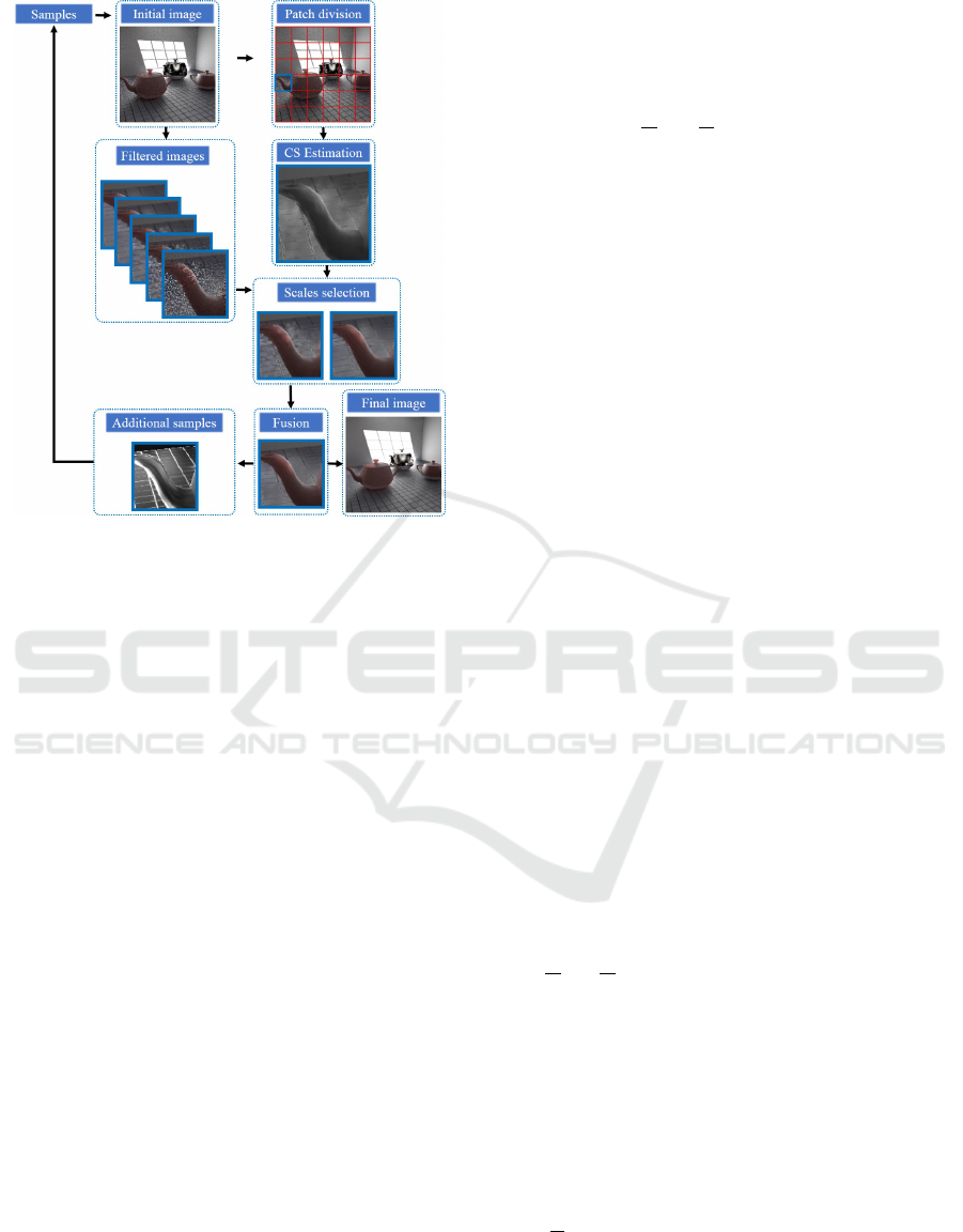
Figure 1: The framework of our algorithm.

motion lead to a shear in the transform domain, and

they introduced a sheared reconstruction ﬁlter to re-

duce the sampling rates. Sen et al. (Sen and Darabi,

2011) ﬁrst introduced the idea of accelerating Monte

Carlo renderings with CS. They ray-traced only a sub-

set of pixels selected by a Poisson-disk distribution,

which provided a speedup over conventional tech-

niques. The missing pixels were then estimated by

a CS solver. Besides, they noticed that the sparsity

of signal goes up as the dimensionality of signal in-

creases. In these cases, high dimensional effects such

as motion blur and depth of ﬁeld are improved by inte-

grating down to obtain the ﬁnal image. However, this

method has difﬁculty in simulating scenes with very

complex details, and is not competitive with those ap-

proaches using feature buffers. Most recently, CS is

also employed to reduce noise artifacts in direct PET

image reconstruction (Vaquer et al., 2016) and the

memory footprint for the scalar ﬂux (Dominik et al.,

2014).

3 COMPRESSED SENSING

Although compressed sensing is not new to computer

graphics, it is rarely applied to improve the quality of

Monte Carlo Renderings. The key idea of compressed

sensing is that a signal can be perfectly reconstructed

if it is sparse in a transform domain. Assuming that

there is a N-dimensional signal x which is to be re-

constructed from M-dimensional sampling signal y,

the CS states that the sampling process is written as:

y = Φx (1)

Where Φ is a M ×N sampling matrix (M < N). In this

paper, the image is divided into patches with a ﬁxed

resolution of

√

N ×

√

N, and each patch performs a

single process of calculating the reconstructed values.

In other words, the local statistics of N pixels is esti-

mated by M pixels.

Typically, it is impossible to reconstruct x from y

with the previous Nyquist-Shannon theorem, because

the band-limit is not met. However, since the CS as-

sumes that x is K-sparse in a transform domain, the

coefﬁcients of x in a transform domain are written as:

θ = Ψ

−1

x (2)

Where Ψ is the N ×N transform basis (or compres-

sion basis). In this case, θ has at most K non-zero

values, which is called the sparsity of the signal in the

compressed basis. Consequently, it is able to elimi-

nate many elements that do not have sparse proper-

ties, and the sampling equation is written as:

y = Φx = ΦΨθ = Aθ (3)

Where A = ΦΨ is a M × N measurement matrix.

Given y and A, θ should be reconstructed if the above

linear system could be solved. Unfortunately, previ-

ous methods such as least squares failed to do this

because M < N and thus the system is undetermined.

In this case, CS algorithms solve the system correctly

as long as some constraints are met. One is that the

sampling number M is twice larger than the sparsity of

the signal (M > 2K). Another one is that the measure-

ment matrix A meets the Restricted Isometry Condi-

tion (RIC), which requires that the sampling matrix

and compressed basis should be incoherent. As K is

usually much smaller than N, less efforts are taken for

CS to reconstruct the original signal. Pay attention to

the formation of x. As the original patch is composed

√

N ×

√

N pixels, we keep track of them with a col-

umn vector of size N ×1, and solve the linear system

for each patch uniquely.

The main challenge is how to select a suitable

sampling matrix Φ and a compressed basis Ψ. There

are many choices such as Gaussian sampling ma-

trix and Bernoulli sampling matrix. Here, since

the Gaussian matrix is uncorrelated with most com-

pressed bases, it is adopted to construct Φ, where

each element of Φ accords with a normal distribution

N(0,

). Besides, Gaussian sampling matrix avoids

the extra sharpening procedure, which is used by Sen

et al. (Sen and Darabi, 2012) as they used a Poisson-

disk distribution to produce y. For the compressed

basis, Discrete Cosine Transform (DCT) is adopted

Removing Monte Carlo Noise with Compressed Sensing and Feature Information

147

in this paper as it outperforms in image processing ar-

eas.

To solve Equation 3, many fast CS algorithms

have been proposed to ﬁnd an approximate solution.

Herein, we employed the Orthogonal Matching Pur-

suit (OMP) since it is simple while effective. The

key idea of OMP is to ﬁnd the representative columns

(atoms) of A that are most related with the sampling

signal y. In this paper, we do not explain OMP details

since it has been widely used, and we just use it to

solve Eq. (3). Readers are encouraged to read related

works for further information about OMP.

Once the linear system is solved, the reconstructed

values can be computed through an inverse transform.

For our method, the reconstructed values are further

used to estimate per-pixel error, which ﬁnally directs

the selection of suitable ﬁlters.

4 ALGORITHM OVERVIEW

Adaptive rendering algorithms that use feature buffers

are extremely effective at removing noise, especially

for scenes that contain very complex details. How-

ever, previous methods usually perform sophisticated

error analyses such as SURE estimator to select an

appropriate ﬁlter, which is unreliable at low sampling

rates. In these cases, many ﬁne details may be lost.

In this paper, the CS is applied to reconstruct pixel

values, which are then used to perform a robust error

analysis.

Our framework is illustrated in Fig. 1. An ini-

tial image x is ﬁrst generated with a small number of

samples. The initial image is divide into patches with

a ﬁxed resolution, and each patch constructs its sam-

pling signal y = Φx. Given the sampling signal y and

measurement matrix A, we calculate the coefﬁcients

θ in the compressed basis through OMP algorithm,

and then take an inverse transform to reconstruct pixel

vales x = Ψθ. Intuitively, the reconstructed values re-

duce the coherence between pixels, and thus they are

less inﬂuenced by neighbors that have a different na-

ture.

After computing the reconstruct pixel values x

with OMP, each pixel is ﬁltered over a discrete set of

ﬁlters with varying parameters to produce the candi-

date ﬁltered value F (Sec.5). The difference between

x and the F is estimated as the pixel error. In gen-

eral, the potential ﬁlter bank is rather large that it is

intractable to ﬁnd the optimal one. In this case, we

carefully choose two ﬁlters with the smallest errors,

and then compute a weighted average of them for out-

put. In particularly, the reconstructed values are pre-

ﬁltered, which allows for producing smooth details.

Finally, if more sample budget is available, a heuristic

metric is proposed to allocate more samples in regions

with larger errors.

5 FILTER SELECTION

To combine pixel colors with feature buffers, the

Cross-bilateral weight is computed for each pixel, and

the ﬁltered value of pixel p is computed as:

F(p) =

N(p)

∑

q∈w(p)

W (p,q)I(q) (4)

Where N(p) =

∑

q∈w(p)

W (p,q) is a normalization

factor. W (p,q) is the contribution of q contributes to

p. I(q) is the input pixel color for pixel q.

5.1 Feature Distance

In this paper, the surface normals, albedo colors and

depths are used to form the feature buffers, and the

feature weight between pixel p and q is computed as:

(p,q) = exp

−

D( f

−f

)

2σ

(5)

Where σ

denotes the standard deviation of the i fea-

ture and D( f

− f

) is the feature distance between

these two pixels. Since the distributed effects such as

motion blur may lead to noisy features, using the sam-

ple means of feature directly can result in inaccurate

results. Thus, a normalized distance is computed as:

D( f

− f

) =

− f

−(var

+ var

ipq

)

τ(var

+ var

)

(6)

Where f

and var

are the sample mean and vari-

ance of the i feature for pixel p, respectively. var

ipq

min(var

,var

) and τ is a user parameter that con-

trols the sensitivity of feature differences. Intuitively,

larger τ causes a more aggressive ﬁltering. In particu-

larly, varying values of τ are designed for different ﬁl-

ters in the ﬁlter bank, which make a balance between

sensitivity to noise and detail ﬁdelity.

The advantages of our normalized distance are

twofolds: First, for a pixel with strong motion blur

or depth of ﬁeld effects, large variances tend to be

generated. Thus D( f

− f

) is relatively small and

the ﬁltering weight increases even when the fea-

tures are far apart. Second, a variance cancellation

term (var

+ var

ipq

) is subtracted to remove the bias

caused by noisy features. Finally, the ﬁlter weight is

computed as:

W (p,q) = exp

−

|p−q|

2σ

exp

−

|I(p)−I(q)|

2σ

∏

i=1

(p,q) (7)

GRAPP 2018 - International Conference on Computer Graphics Theory and Applications

148

Figure 2: Feature buffer and the scale selection map. Our

approach make a nice trade-off between robustness to noise

and ﬁdelity to image detail.

Where σ

and σ

are the stand deviation parameters

of the spatial and range kernels, respectively.

5.2 Filters Averaging

Previous methods typically choose a single ﬁlter from

the pre-deﬁned ﬁlter bank for output. However, as

the potential size of the ground truth is very large, it

is intractable to select the optimal one. Furthermore,

choosing the appropriate parameters of ﬁlter bank for

different scenes is challenging. In this paper, this

problem is addressed by evaluating the errors of the

ﬁltered colors on a per-pixel basis, which allows us to

obtain a better choice.

Assuming the reconstructed value using CS solver

at pixel p is interpreted as x

, the ﬁltered error of the

i ﬁlter is estimated as:

Err

= 2

−F

(p)|

(p) + ε

+ σ

(8)

Where F

(p) denotes the ﬁltered value of pixel p using

the i ﬁlter in the ﬁlter bank. σ

is the sample variance

and ε is a small number to prevent division by zero.

Eq. 8 focuses on two issues. First, the difference be-

tween the ﬁltered value F

(p) and reconstructed value

is estimated to measure the size of the optimal ﬁl-

ter. Second, the variance term is considered to obtain

a more smooth result. For pixels with complex geom-

etry details, large scale ﬁlters produce a large differ-

ence term, and thus they lead to large errors. For sim-

ple pixels, however, the reconstructed values tend to

be smoother. In these situations, large scale ﬁlters re-

sult in small errors. In practice, we use the Y channel

of CIE1934(XYZ) color space to compute the ﬁltered

error.

After calculating the ﬁltered error of each candi-

date ﬁlter, a weighted average of two ﬁlters is com-

puted. For each pair of consecutive ﬁlters, the sum of

their cumulative error Err

+Err

i+1

is computed. The

single pair that returns the smallest value is selected.

Then, the weighted average is computed as:

F(p) =

∑

i+1

j=i

exp

−

Err

(p)

∑

i+1

j=i

exp

−

Err

(9)

Figure 3: Sampling density map.

Where i = arg min

i=1,2,...L−1

{Err

+ Err

i+1

} and L is

the size of ﬁlter bank. Finally, F(p) is used to update

pixel.

Fig. 2 demonstrates our scale selection map,

which is denoted by the i ﬁlter for each pixel. It is

obviously that our approach make a nice trade-off be-

tween robustness to noise and ﬁdelity to image detail,

where small scale ﬁlters concentrate on complex re-

gions and large ones tend to be used in simple regions.

5.3 Adaptive Sampling

To perform the adaptive sampling process, the esti-

mated error is chosen as a feedback to direct the sam-

pling function:

(Err

+ Err

i+1

) + σ

F(p)

+ n

(10)

Where F(p)

is the squared luminance of the

weighted average value, and n

is the number of sam-

ples that have already been distributed in pixel p.

Thus, pixel p obtain kS

∑

) samples if there are

k samples available. The sampling density map is

shown in Fig. 3. It shows that samples concentrate

on regions with complex details and more noise.

6 ANALYSES

Fig. 4 compares our method with global ﬁlters of

each scale. For small scale ﬁlters (scale = 0,1),

noise is hard to be removed. For large scale ﬁlters

(scale = 4,8), however, edge details on the window

are over smoothed. It is obviously that our method

make a nice trade-off between robustness to noise and

ﬁdelity to image details.

Removing Monte Carlo Noise with Compressed Sensing and Feature Information

149

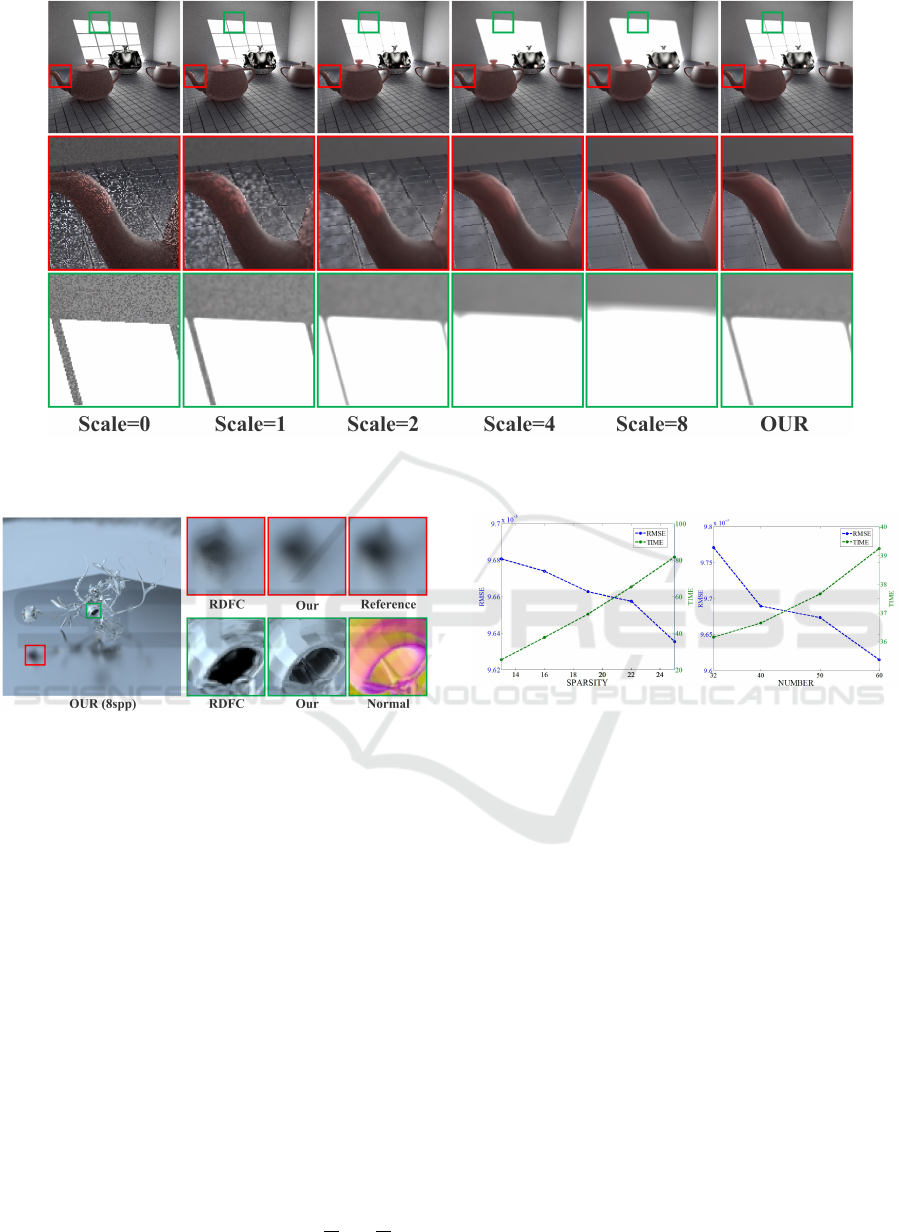
Figure 4: The comparison between our method and global ﬁlters. Our method adjusts ﬁlter scales in a consecutive manner

and removes noise while preserving details.

Figure 5: The comparison between our method and RDFC

method. RDFC does not estimate ﬁlter errors accurately at

low sampling rates and thus over blurs image details. Our

method returns a better result.

One key advantage of the new approach is the ro-

bustness of error analysis at low sampling rates. For

previous error estimators such as SURE, excessive

variance tends to be generated in the color buffer, and

thus they are unreliable at low sampling rates. In such

situations, edge details are hard to be preserved. Fig.

5 shows a scene with glossy materials. It is obvi-

ously that RDFC frequently shows ringing artifacts

caused by its inaccurate error estimation. The second

row of insets further highlights the contribution of our

CS framework. As the image is sparse in the trans-

form domain, the reconstructed values reduce the co-

herence between pixels greatly. Thus, the difference

between the ﬁltered value and reconstructed value re-

turns a more reliable error estimation. Pay attention to

the structure edges, RDFC over blurs the details while

our method keeps the ﬁdelity.

For the proposed approach, the image is divided

into patches with a ﬁxed resolution of

√

N ×

√

N pix-

Figure 6: Visualizations of different sparsity values and

sampling numbers. Larger values lead to smaller errors,

however, more time is also needed.

els, and there are two key parameters to be deter-

mined: sparsity K and sampling number M. For the

current implementation, N is set to 64. The visual-

izations of these two parameters are shown in Fig. 6,

which uses the scene in Fig. 5. As shown in the ﬁgure,

large values for both parameters lead to smaller errors,

however, the time also increases greatly. For our cur-

rent implementation, K and M are set to 20 and 50

respectively, and the experimental results show that

they outperforms in most cases.

7 RESULTS

The proposed approach was implemented on the top

of PBRT-V2 (Pharr and Humphreys, 2010). The CS

framework was implemented in MATLAB2013 using

the paralleling computing toolbox and then integrated

into PBRT. All the images were rendered by an Intel

Core 2.4 GHz CPU with 8 GB of memory. In addi-

GRAPP 2018 - International Conference on Computer Graphics Theory and Applications

150

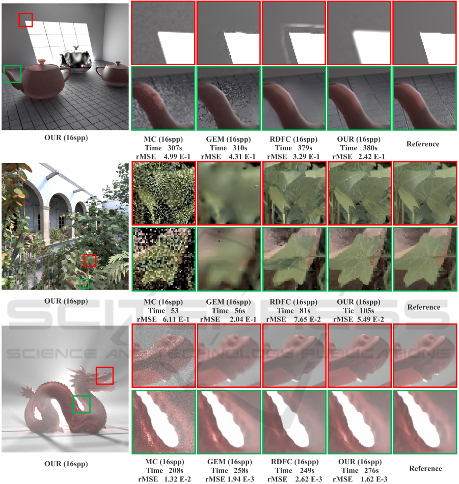
Figure 7: Comparisons between our method and previous methods. MC typically produces considerable noise. GEM removes

noise effectively, however, it tends to over blur images. RDFC presents visually pleasing results. Nonetheless, some ﬁne

details may be lost at low sampling rates.

tion, we wrote a GPU-based Cross-bilateral ﬁlter to

accelerate the algorithm. For our method, the ﬁlter

bank was constructed with spatial-varying parameters

= 0,1, 2,4,8 and τ = 0.125, 0.5,1,2, 5. The pa-

rameters of features were set as for σ

= 0.2 albedo,

= 0.3 for depth and σ

= 0.4 for normal.

7.1 Scenes

We compared our method with three previous meth-

ods. The ﬁrst one is the naive Monte Carlo method

(MC) that is available from PBRT render (Pharr and

Humphreys, 2010). The second method is the greedy

error minimization algorithm (GEM) proposed by

Rousselle et al. (Rousselle et al., 2011), and the

gamma parameter was set to 0.2 as suggested in the

Removing Monte Carlo Noise with Compressed Sensing and Feature Information

151

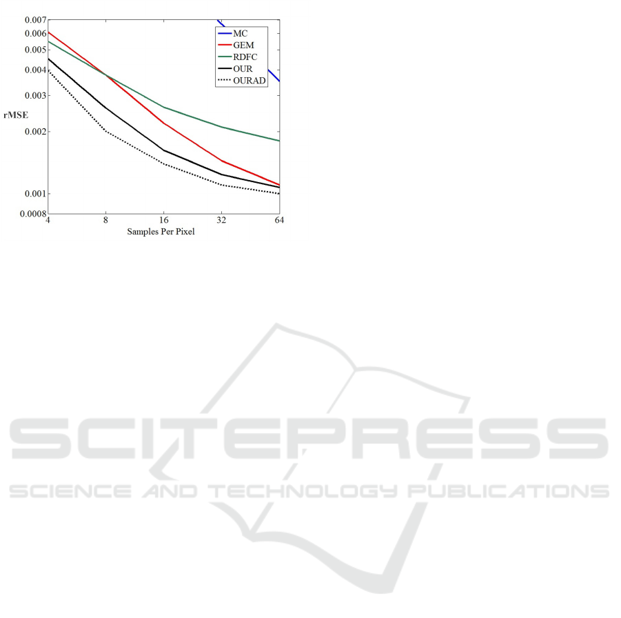
Figure 8: Convergence plots for different methods.

original paper. The last method is a feature-based

method (RDFC) (Rousselle et al., 2013). The win-

dow size was set to 10 and all the other parameters

were default values. For all of the tested scenes, both

visual image quality and relative MSE (rMSE) were

tested with the same sample number. We adopted the

rMSE proposed by Rousselle et al. (Rousselle et al.,

2011): (img −re f )

/(re f

+ε). re f is the pixel color

in the reference image, and ε = 0.01 is a small number

to prevent division by zero.

In Fig. 7, three scenes are compared and all the

images were rendered at a resolution of 800 ×800

pixels. The ﬁrst ROOM-IGI scene is a challeng-

ing scene rendered by instant global illumination al-

gorithm, where most of the illumination is indirect.

The image produced by MC contains considerable

noise both on the wall and spout of the teapot. GEM

removes noise greatly on the wall, however, it fre-

quently presents splotches. RDFC returns clearer de-

tails, but it over blurs the edges on the ﬂoor. Besides,

RDFC also introduces visible artifacts on the window.

Compared with these methods, our method generates

a relatively noise-free image while faithfully preserv-

ing details.

The SANMIGUEL is a path-traced scene with

very complex geometries. Again, MC presents severe

noise, and GEM over blurs the textures because of the

symmetric kernels. Compared with MC and GEM,

RDFC preserves the structure details and removes the

noise. However, as the SURE-error estimation is in-

accurate at low sampling rates, some ﬁne details are

lost. Meanwhile, the features are not weighted ap-

propriately by RDFC and thus it fails to keep the ﬁne

details, while our method yields a smoother result and

preserves foliage details very well.

The DRAGONFOG scene includes many partic-

ipating media, and is rendered using PBRTs photon

mapper. GEM removes most noise on the smooth

regions, but it generates ambiguous details on the

mouth. Although RDFC and our method present the

visually equal results, we found that RDFC tends to

produce darker details for this scene and thus results

in a larger rMSE. Meanwhile, our result is closer to

the ground truth.

Fig. 8 presents the log-log convergence plots for

the dragonfog scene. We demonstrate the results

for naive Monte Carlo method (MC in blue), GEM

method (Rousselle et al., 2011) (GEM in red), RDFC

method (RDFC in green), our work using uniform

sampling (OUR in black), and our work with adap-

tive sampling (OURAD in dotted black). RDFC out-

performs GEM at low sampling rates. However, it

performs worse at high sampling rates since it tends

to produce darker details. Although higher sam-

pling number and sparsity could reduce the errors,

experimental results demonstrate that our current set-

tings are able to handle most cases. This ﬁgure

demonstrates that our CS-based weighted averaging

of candidate ﬁlters consistently returns pleasing re-

sults. Moreover, our adaptive sampling process fur-

ther reduces the rMSE.

7.2 Limitations

There are some limitations for the proposed algo-

rithm. First, the initial image is divided into patches

that each one corresponds to a ﬁxed resolution. It lim-

its the quality of rendering results, where patches with

varying sizes are more suitable. Second, similar to

previous methods, ﬁlters based on features are prone

to blurring structure details that are not well repre-

sented by these features. Novel features such as caus-

tics, visibility and feature gradient help to further re-

move noise. Feature gradient, for instance, prevents

restrictive ﬁlter weights and preserves edge details.

For our current implementation, we only use surface

normal, albedo color and depth since they outperform

in most cases. Finally, little theoretically sound con-

tributions are presented for the compressed sensing.

Improvements on the sampling basis and compressed

basis can further improve the rendering quality.

8 CONCLUSIONS AND FUTURE

WORKS

A novel rendering algorithm has been presented to

address the noise artifacts of Monte Carlo rendering.

A robust error estimation procedure is proposed by

exploring the sparsity with compressed sensing theo-

rem. Pixel values are reconstructed in a transform do-

main, which returns a sparse nature and facilitates the

GRAPP 2018 - International Conference on Computer Graphics Theory and Applications

152

estimation of ﬁlter errors. We use a normalized dis-

tance to measure the difference between features and

then return more reasonable ﬁlter weights. To obtain

the optimal ﬁlter scale, two candidate ﬁlters are se-

lected to determine a weighted average value on a per-

pixel basis. Meanwhile, an iterative sampling process

is also adopted to distribute more samples in regions

with higher estimated errors. Through combining CS

results with feature information, our method provides

signiﬁcant improvements both in visual and numeri-

cal quality.

This paper raises several interesting issues for our

future work. First, the sparsity of the image goes up as

the number of considered dimensions increases. This

allows us to explore the improvements of speciﬁc dis-

tributed effects such as depth of ﬁeld and motion blur.

For example, by integrating samples along the dimen-

sion of time, motion blur is improved with pixel val-

ues reconstructed in the transform domain. Second, a

better transform basis that is more suitable for Monte

Carlo renderings should be directed through combin-

ing with recent advances in Compressed Sensing. In

addition, we intend to apply this work to related areas

such as wave rendering.

REFERENCES

Bako, S., Vogels, T., Mcwilliams, B., Meyer, M., Nov

aK,

J., Harvill, A., Sen, P., Derose, T., and Rousselle,

F. (2017). Kernel-predicting convolutional networks

for denoising monte carlo renderings. ACM Trans.

Graph., 36(4):97:1–97:14.

Dominik, R., Thomas C., B.-L., Thomas, K., and Andr, F.

(2014). Compressed sensing for reduction of noise

and artefacts in direct pet image reconstruction. Z.

Med. Phys, 24(1):16–26.

Durand, F., Holzschuch, N., Soler, C., Chan, E., and Sillion,

F. X. (2005). A frequency analysis of light transport.

ACM Trans. Graph., 24(3):1115–1126.

Egan, K., Tseng, Y.-T., Holzschuch, N., Durand, F.,

and Ramamoorthi, R. (2009). Frequency analysis

and sheared reconstruction for rendering motion blur.

ACM Transactions on Graphics (SIGGRAPH 09),

28(3).

Hachisuka, T., Jarosz, W., Weistroffer, R. P., Dale, K.,

Humphreys, G., Zwicker, M., and Jensen, H. W.

(2008). Multidimensional adaptive sampling and re-

construction for ray tracing. ACM Trans. Graph.,

27(3):33:1–33:10.

Kalantari, N. K., Bako, S., and Sen, P. (2015). A machine

learning approach for ﬁltering monte carlo noise.

ACM Trans. Graph., 34(4):122:1–122:12.

Kalantari, N. K. and Sen, P. (2013). Removing the

noise in monte carlo rendering with general image

denoising algorithms. Computer Graphics Forum,

32(2pt1):93102.

Lehtinen, J., Aila, T., Chen, J., Laine, S., and Durand,

F. (2011). Temporal light ﬁeld reconstruction for

rendering distribution effects. ACM Trans. Graph.,

30(4):55:1–55:12.

Li, T.-M., Wu, Y.-T., and Chuang, Y.-Y. (2012). Sure-

based optimization for adaptive sampling and recon-

struction. ACM Trans. Graph., 31(6):194:1–194:9.

Moon, B., Carr, N., and Yoon, S.-E. (2014). Adaptive

rendering based on weighted local regression. ACM

Trans. Graph., 33(5):170:1–170:14.

Moon, B., Iglesias-Guitian, J. A., Yoon, S.-E., and Mitchell,

K. (2015). Adaptive rendering with linear predictions.

ACM Trans. Graph., 34(4):121:1–121:11.

Moon, B., Jun, J. Y., Lee, J., Kim, K., Hachisuka, T., and

Yoon, S. (2013). Robust image denoising using a vir-

tual ﬂash image for Monte Carlo ray tracing. Comput.

Graph. Forum, 32(1):139–151.

Overbeck, R. S., Donner, C., and Ramamoorthi, R. (2009).

Adaptive wavelet rendering. ACM Trans. Graph.,

28(5):140:1–140:12.

Pharr, M. and Humphreys, G. (2010). Physically Based

Rendering: From Theory to Implementation. Morgan

Kaufmann Publishers Inc., San Francisco.

Rousselle, F., Knaus, C., and Zwicker, M. (2011). Adaptive

sampling and reconstruction using greedy error mini-

mization. ACM Trans. Graph., 30(6):159:1–159:12.

Rousselle, F., Knaus, C., and Zwicker, M. (2012). Adaptive

rendering with non-local means ﬁltering. ACM Trans.

Graph., 31(6):195:1–195:11.

Rousselle, F., Manzi, M., and Zwicker, M. (2013). Robust

Denoising using Feature and Color Information. Com-

puter Graphics Forum.

Sen, P. and Darabi, S. (2011). Compressive rendering: A

rendering application of compressed sensing. IEEE

Transactions on Visualization & Computer Graphics,

17(4):487–499.

Sen, P. and Darabi, S. (2012). On ﬁltering the noise from

the random parameters in monte carlo rendering. ACM

Trans. Graph., 31(3):18:1–18:15.

Soler, C., Subr, K., Durand, F., Holzschuch, N., and Sillion,

F. (2009). Fourier depth of ﬁeld. ACM Trans. Graph.,

28(2):18:1–18:12.

Vaquer, P. A., McClarren, R. G., and McClarren, R. G.

(2016). A compressed sensing framework for monte

carlo transport simulations using random disjoint tal-

lies. Journal of Computational and Theoretical Trans-

port, 45(3):219–229.

Zwicker, M., Jarosz, W., Lehtinen, J., Moon, B., Ra-

mamoorthi, R., Rousselle, F., Sen, P., Soler, C., and

Yoon, S.-E. (2015). Recent advances in adaptive sam-

pling and reconstruction for Monte Carlo rendering.

Comput. Graph. Forum, 34(2):667–681.

Removing Monte Carlo Noise with Compressed Sensing and Feature Information

153