Hyperspectral Compressive Sensing Imaging Via Spectral Sparse

Constraint

Qi Wang

, Hong Xu

, Lingling Ma

1,*

, Chuanrong Li

, Yongsheng Zhou

and Lingli Tang

Key Laboratory of Quantitative Remote Sensing Information Technology, Academy of Opto-Electronics,

Chinese Academy of Sciences, Beijing, 100094, China

High Technology Research and Development Center, Ministry of Science and Technology, Beijing 100862, China

Keywords: Compressive Sensing, Hyperspectral Imaging, Sparse Representation, Dictionary Learning, Reconstruction

Algorithm.

Abstract: The existing algorithms to reconstruct hyperspectral compressive sensing images mainly use the sparse

property of spatial information and some simple non-adaptive spectral constraint such as the low-rank

property. However, these strategies cannot remove the spectral redundancy efficiently and a new method to

make full use of the abundant redundancy of spectral information and improve the quality for hyperspectral

CS reconstruction is necessary. A new CS sampling and reconstruction model based on spectral sparse

representation was proposed in this paper. The spectral sparse dictionary was constructed from training

samples to enhance the effect of sparse representation and the total variation constraint of spatial images was

also considered to further enhance the precision during the reconstruction. The experiment to reconstruct

AVIRIS hyperspectral images of 200 bands show that the hyperspectral image was almost perfectly

reconstructed at 25% sampling rate and the spatial and spectral precision was higher than traditional methods

which only adopt the spatial sparsity and simple non-adaptive spectral constraint in the same condition.

1 INTRODUCTION

Hyperspectral remote sensing technique has the

ability to acquire and analyze the physical and

chemical properties of land surface objects. Over the

past 30 years it has witnessed a great progress in

various fields such as atmosphere monitoring, ocean

monitoring, mineral exploration, precision agricul-

ture and target detection. However, hyperspectral

images have much larger amount of data which makes

data transmission, storage and onboard processing

more difficult. Furthermore, the optics system will

also become more complicated and costly with the

improvement of resolution. As far as the traditional

imaging system based on Nyquist sampling theory is

concerned, it is almost impossible to conquer the

contradiction between high efficiency and high

resolution demand. Therefore, new theory is expected

to be developed so as to promote more efficient

application of hyperspectral remote sensing.

As a novel theory in signal processing,

compressive sensing (CS) theory which integrates

compression and sampling process has drawn much

attention in many fields including remote sensing

imaging (Donoho, 2006). By concerning the sparse

characteristic of the object, images can be

reconstructed from very few measurements.

Therefore the size and complexity, as well as the on-

orbit computational cost of the CS imaging system is

much lower than conventional systems, making it a

very promising application in the remote sensing (Li,

2014). A. Wagadarikar (2008), Thomas A. Russell

(2012), and J. Wu (2014) have developed various CS

spectral imaging systems respectively.

The images of CS imaging system are

reconstructed from compressive measurements by

solving specific optimization problem. The sparse

characteristics of target signal is the foundation of CS

reconstruction: the better the signal is sparsely

represented, the higher reconstruction precission

would be obtained. The total variation (TV) model

based on the sparsity of two dimensional discrete

gradient was widely used to reconstruct spatial

images (Combettes, 2014). However, in the

hyperspectral remote sensing imaging which

demands for higher compression rate, the

Wang, Q., Xu, H., Ma, L., Li, C., Zhou, Y. and Tang, L.

Hyperspectral Compressive Sensing Imaging via Spectral Sparse Constraint.

DOI: 10.5220/0006664202730278

In Proceedings of the 6th International Conference on Photonics, Optics and Laser Technology (PHOTOPTICS 2018), pages 273-278

ISBN: 978-989-758-286-8

273

reconstruction effect of non-adaptive total variation

model is usually dissatisfied. There is strong

correlation among the bands of hyperspectral image.

Regarding to this characteristic, several constraint

models using spectral correlation had been proposed.

Zhang et. al. extended the traditional two-

dimensional TV model to 3 dimensions in order to

reconstruct hyperspectral images (Zhang, 2014).

Feng et. al. (2012) used the current reconstructed

band as the reference to predict the following band.

Liu et. al. (2011) presented the hyperspectral

reconstruction algorithm based on the prediction of

the residual vector. Golbabaee et. al. (2012) applied

the low-rank property of hyperspectral data bands and

reconstructed the image by adding the nuclear norm

to the constraint model. Jia et. al. (2014) put forward

a structural-relation-based model via researching the

spectral statistical correlation of hyperspectral image.

These spectral correlation models do enhance the

reconstruction precision to some extent, but the

spectral constraint models are relatively simple and

non-adaptive, thus the detailed spectral information is

difficult to be reconstructed correctly at a low

sampling rate. This shortage is more notable for the

hyperspectral scenes with a wider spectral range and

more bands of data.

Actually, most of the earth surface spectrum

possesses piecewise smooth property with a large

amount of redundant information. The spectral

information redundancy is usually more abundant

than that of the complex spatial information and is not

well removed using the available methods such as

neighboring band prediction or low-rank

minimization of the HSI data. On the other hand, the

sparse representation theory suggests that, the signals

can be precisely represented by very few atoms from

some kinds of dictionaries that can highly reduce the

information redundancy. Recently some researchers

applied the sparse representation theory in the

hyperspectral fields such as spectral classification,

unmixing, and reconstruction (Zare, 2012, Charles,

2011, Wang, 2013). By exploiting the spectral sparse

property, researchers obtained better results than

conventional methods, making it an effective way to

process HSI data.

On such basis, the sparse representation theory is

introduced to reconstruct compressive sensing

hyperspectral images in this paper and a new

hyperspectral sampling model is proposed to

precisely reconstruct the images in the CS scheme. In

Section II, the sparse representation theory and the

method of spectral sparse dictionary learning are

discussed. In Section III, the principles of spectral

compressive sensing model and the hyperspectral

image reconstruction algorithm based on the spectral

sparse dictionary are presented. In Section IV, the

experiment of sampling and reconstructing the

AVIRIS scene is conducted, and our method as well

as three different hyperspectral reconstruction

methods is applied in comparison. In Section V, the

content of this paper is concluded and the problems

and prospects are analyzed.

2 SPECTRAL SPARSE

DICTIONARY LEARNING

Suppose x is a signal of length N and D=[d

,…d

]

is a set of basis (also called as dictionary) in the N-

dimensional Euclidean space. If x can be linearly

represented by the L atoms in the dictionary (usually

L<<K, N), then we declaim that x has a sparse

representation in the dictionary D, the sparsity level

is L. That is

, 1,2...

x d K



  



  



(1)

where ε is the residual error of the sparse

representation. (1) can be rewritten in the matrix form:

x Ds





(2)

In which s, called as the sparse coefficient, is the

coordinate vector with only L non-zero elements. The

process to calculate s is called as sparse coding and it

solves the minimization problem:

min , . .s st x Ds

(3)

where || • ||

denotes the number of non-zero

elements and (3) can be solved by several algorithms.

A more important question of the sparse

representation is the way to construct the dictionary.

In the area of signal and image processing, DCT

dictionary, wavelet dictionary and Gabor dictionary

are usually adopted. The atoms in these dictionaries

are fixed and hard to be adjusted adaptively, which

results in the limitation that more efficient and

accurate decomposition is needed for hyperspectral

CS reconstruction. In recent years the adaptive

dictionary training method from the characterized

sample set is developed and used in the sparse

dictionary construction by many researchers. The

dictionary learning method is an adaptive approach

for complex signals and usually achieves a better

result than conventional dictionaries such as DCT and

wavelet. The main idea of dictionary training is to

find a matrix that ensures each sample in the training

PHOTOPTICS 2018 - 6th International Conference on Photonics, Optics and Laser Technology

274

set a sparse representation by such matrix. The

sparsity level and the residual error in the

representation are the optimization goal in the

calculation. For the hyperspectral dictionary

construction in this paper, the spectral sparse

dictionary model is presented as

min . .

W DS st i s L  

(4)

where the matrix W is composed by the column

vectors of spectral sample set that are extracted from

hyperspectral scenes, D and S are the sparse

dictionary and the coefficients to be solved

respectively, and L is the sparsity level control

parameter. The solving process of (4) consists of two

key steps called as sparse coding and dictionary

updating. The sparse coding step is to solve the sparse

coefficients S under the dictionary D and the updating

step is to adjust D according to the new coefficients.

The two steps are executed alternatively until

convergence. Based on the different approach to

realize dictionary updating, a series of dictionary

learning algorithms such as KSVD, MOD and RLS

are presented (Aharon,2006, Mairal, 2009, Skretting,

2010). Here we choose the KSVD algorithm as the

dictionary learning algorithm and fast OMP as the

sparse coding algorithm for their relatively high

accuracy and efficiency (Azimi, 2014).

3 HYPERSPECTRAL SAMPLING

AND RECONSTRUCTION

Suppose the matrix X represents a hyperspectral data

cube, with N=n

spatial pixels and B spectral

bands. The compressive sampling of hyperspectral

object is conducted in the spatial region usually. x

denotes for the column vector with length N expand-

ing from the i-th band image, and y

denotes for the

corresponding measurements. To sample the scene by

the linear mixing matrix P in each band, we have

1 2 1 2

[ , ,..., ] [ , ,..., ]

y y y P x x x

(5)

The usual way to solve (5) is to reconstruct each

spatial image in the constraint of total variation and

adjust the solution based on the spectral correlation

model. As pointed before, the spectral sparse property

with a large amount of information redundancy is not

exploited sufficiently in this model. Therefore, we

propose a new sampling scheme in the spectral region.

denotes the spectral data vector with length B of the

i-th spatial pixel and y

denotes the corresponding

compressive measurements. The sampling process is

applied in the whole spatial region, that is

1 2 1 2

[ , ,..., ] [ , ,..., ]

y y y P

  



(6)

And the hyperspctral scene is reconstructed based

on (6).

In the spectral sparse model of Section II, the

spectral signal in (6) can be decomposed as the

product of sparse dictionary and coefficients, that is

, 1,2,...,

Ds i N





(7)

Define matrix A=PD and put (7) into (6):

i i i

y PDs As

(8)

And the sparse coefficients s

is determined from

solving the optimization problem

min , . .

i i i

s st y As

(9)

As the sparse representation error is unavoidable,

(9) is presented as an unconstrained optimization

problem with the regularizer β

min

i i i

y As s





(10)

The optimization of the l

norm is a NP hard

problem. Therefore we use smooth Gaussian function

to approximate the l

norm and convert the problem

to classical convex optimization problem which can

be solved via gradient descent pursuit algorithm. The

detailed steps are presented in (Mohimani, 2007).

Solve (10) for the spectrum in each pixel and

calculate the reconstructed spectrum via (7) and

arrange all the spectrum into a three dimensional

matrix to construct the raw reconstructed

hyperspectral data cube X

. The accuracy of spatial

information of the reconstructed image is hard to

guarantee with the spectral constraint only. Therefore

the raw reconstructed data is revised in the constraint

of total variation to solve the optimization problem

with the regularizer β

min

j j j

x x x









(11)

in which x

is the j-th band spatial image of X

and

x’

is the revised image in the constraint of total

variation. The TV norm represents for

1i i i n i

x x x x x



   



(12)

Solve (12) for each band in X

to construct the

data cube X’ by applying the algorithm in

(Chambolle,2004) and further revise the spectrum via

Hyperspectral Compressive Sensing Imaging via Spectral Sparse Constraint

275

solving the optimization problem which is similar to

(10):

2 2 0

min

i i i i i

y As s s s





   

(13)

Calculate (11) and (13) alternatively to revise

spatial and spectral solution of the reconstructed

scene until the convergence is reached:

0.001





(14)

4 EXPERIMENTS AND RESULTS

Spectral Dictionary Learning: The spectral data from

the remote sensing images acquired by AVIRIS

hyperspectral imagery at the range of 0.4-2.5 μm is

selected as the dictionary learning samples. The

sample set contains 5000 spectrums from 38 types of

ground objects in the scene Indian pines, Salinas,

Cuprite and Kennedy Space Center. Since some

bands are influenced by water vapor absorption, 24

bands are discarded and the data of 200 bands are

used eventually. The spectral data is normalized to

avoid the difference of the intensity in the different

scene and some types of training samples are shown

in Fig. 1. In the dictionary training algorithm we set

the sparsity level L=5, the iteration times T=30, and

the number of atoms K=400. The parameters are

selected from many experiments considering both the

efficiency and precision of the algorithm, while the

influence of the parameter changing on the dictionary

and the method to decide the best parameter is yet to

be further studied.

Experiment 1: The experiment scene to be

reconstructed is selected from the area of Indian Pines

containing 128*128 pixels (the test area is not

included in the training set). The compressive

sampling is conducted to the scene by the random

Bernoulli matrix that has good incoherence property

and is sustainable by hardware. The sampling rate is

25%, and Gaussian noise of 40dB SNR is added to

the measurements. The original data of 200 bands are

compressed to 40 bands after sampling.

The algorithm presented in Section III is applied

to reconstruct the hyperspectral scene from the

compressive measurements. The regularizers of β

, β

and β

are set to 0.4, 0.1, and 0.1 respectively. In

contrast, three different hyperspectral CS

reconstruction algorithms are also tested including

TV algorithm in (Combettes,2004), TVSS algorithm

in (Liu,2011) and TVNU algorithm in

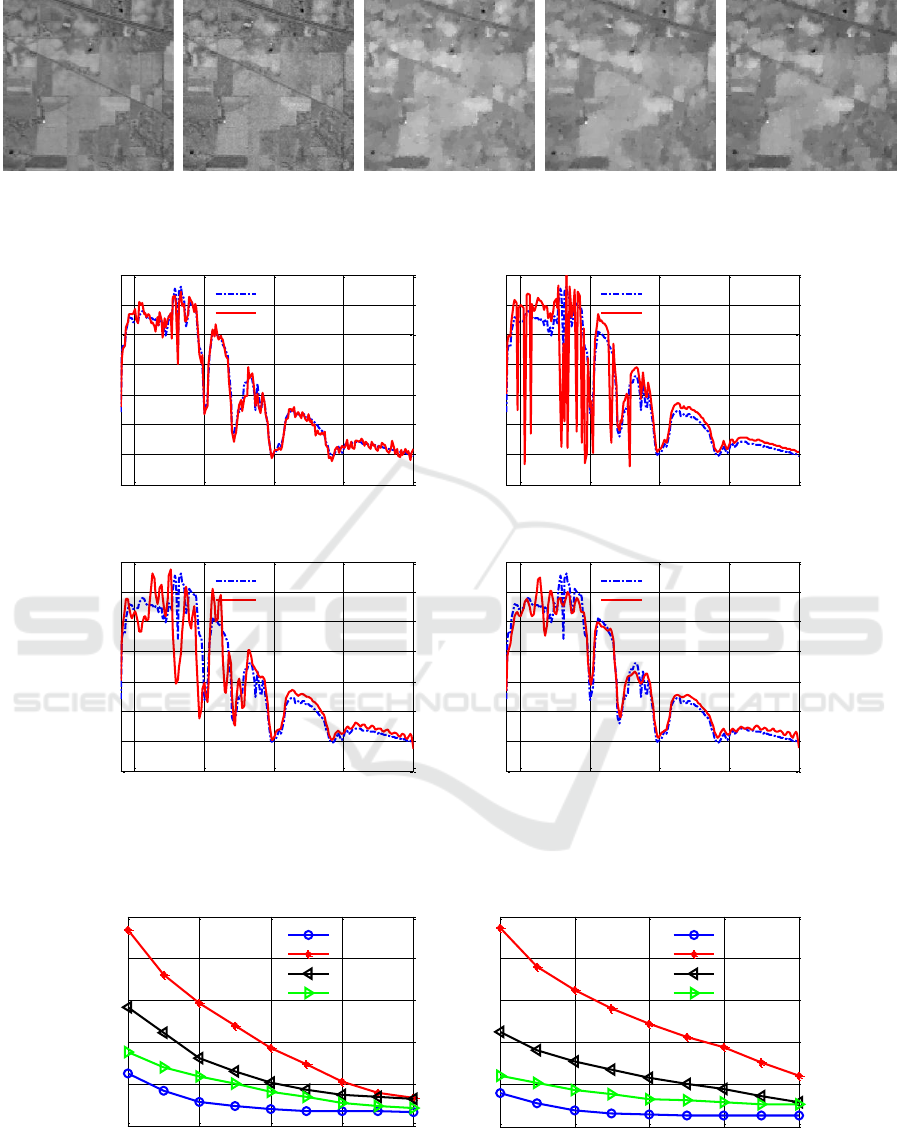
(Golbabaee,2012). Fig. 2 shows the reconstructed

image of the 100th band via the four algorithms in the

same experimental condition. The quality of the

reconstructed image by the proposed method is

significantly better that other algorithms and it

effectively avoids the over-smoothing problem

blurring the image details by TV constraint

algorithms.

Figure 1: Some types of spectrum in the training set

extracted from AVIRIS data containing 200 valid bands.

The spectral intensity is normalized.

The spectral curve of corn in the scene is

compared before and after reconstruction in Fig.3 via

different algorithms. The reconstructed spectrum by

the proposed method achieves very high accuracy

with little deviation. In contrast, the TV algorithm

fails at some bands and makes the spectrum

discontinuous due to the lack of constraint in the

spectral region. The TVSS and TVNU algorithm with

spectral constraint maintain the continuity of the

reconstructed spectrum to some extent, but there are

apparent errors in some details especially at the

wavelength 0.5-1.0μm where the spectrum has a wide

fluctuation.

Experiment 2: Change the sampling rate and

reconstruct the hyperspectral scene via different

algorithms. The sampling rate is set from 10% to 50%.

To assess the reconstruction precision, two

parameters represented for space and spectrum

respectively are calculated for each reconstructed

hyperspectral scene. One is the mean value of the root

square error (RMSE) of each spatial band and the

other is the mean value of the spectral angle (MSA)

between the reconstructed spectrum and the original

one. The result is shown in Fig.4. The precision of the

reconstructed scene via the proposed method is better

than other algorithms in both spatial region and

spectral region. The advantage of our method is more

dominant especially at low sampling rate due to the

precise sparse constraint in the spectral region.

0.5 1 1.5 2 2.5

0.05

0.1

0.15

0.2

Wavelength(μm)

Normalized intensity

Woods

Corn

Alfalfa

Grass-pasture

Wheat

PHOTOPTICS 2018 - 6th International Conference on Photonics, Optics and Laser Technology

276

(a) (b) (c) (d) (e)

Figure 2: The 100th band reconstructed image from the AVIRIS scene Indian pines via different algorithms from

25%sampling measurements. (a)Original image. (b) Our method. (c)TV algorithm. (d)TVSS algorithm. (e)TVNU algorithm.

(a) (b)

Figure 3: The corn spectrum in the AVIRIS scene Indian pines before and after reconstruction via different algorithms from

25%sampling measurements. (a) Our Method. (b)TV algorithm. (c)TVSS algorithm. (d)TVNU algorithm.

(a) (b)

Figure 4: The quality assessment parameters of the reconstructed hyperspectral image at different sampling rate varying from

0.1 to 0.5 in the same CS experiment. (a) The RMSE value to assess spatial reconstruction quality. (b)The MSA value to

assess spectral reconstruction quality.

0.5 1 1.5 2 2.5

0.02

0.04

0.06

0.08

0.1

0.12

0.14

Wavelength(μm)

Normalized intensity

True spectrum

Reconstructed spectrum

0.5 1 1.5 2 2.5

0.02

0.04

0.06

0.08

0.1

0.12

0.14

Wavelength(μm)

Normalized intensity

True spectrum

Reconstructed spectrum

0.5 1 1.5 2 2.5

0.02

0.04

0.06

0.08

0.1

0.12

0.14

Wavelength(μm)

Normalized intensity

True spectrum

Reconstructed spectrum

0.5 1 1.5 2 2.5

0.02

0.04

0.06

0.08

0.1

0.12

0.14

Wavelength(μm)

Normalized intensity

True spectrum

Reconstructed spectrum

0.1 0.2 0.3 0.4 0.5

0.005

0.01

0.015

0.02

0.025

Sampling Rate

RMSE

Our Method

TVSS

TVNU

0.1 0.2 0.3 0.4 0.5

0.1

0.2

0.3

0.4

0.5

Sampling Rate

MSA

Our Method

TVSS

TVNU

Hyperspectral Compressive Sensing Imaging via Spectral Sparse Constraint

277

5 CONCLUSIONS

Aiming at the problem to utilize the spectral sparse

property in the hyperspectral CS remote sensing

imaging, this paper presents a new sampling and

reconstruction method based on the spectral sparse

representation. By learning the spectral sparse

dictionary to constrain the spectral region in the

reconstruction and optimizing the spatial precision

via total variation constraint, the AVIRIS

hyperspectral scene is reconstructed in very high

quality from 25% compressive measurements, which

provides a new idea to enhance the hyperspectral

sampling efficiency. Compared with other presented

hyperspectral CS reconstruction algorithms, the

reconstruction precision in spatial and spectral region

of our method has a significant superiority in the same

experimental condition.

However, there still exist some problems to be

further studied in order to better apply the new theory.

One is the method of the spectral training sample

construction and dictionary learning. In the

experiment it is found that if the training samples are

extracted from the sensor or the type of ground object

with a great difference from that of the reconstructed

area, the effect of the spectral sparse representation is

significantly affected and the reconstruction precision

decreases. The other one is the realization of spectral

random coding in hardware, for the spectral sampling

scheme is more difficult to realize than spatial

sampling.

ACKNOWLEDGEMENTS

This work is supported by the National Key Research

and Development Program of China under Grant

2016YFB0500402, CAS/SAFEA International

Partnership Program for Creative Research Teams

under Grant 2013AA1229 and the Strategic Priority

Research Program of the Chinese Academy of

Sciences under Grant XDA13030402.

REFERENCES

Donoho, David L, 2006. Compressed sensing. IEEE Trans.

Inform. Theory. 52.4, p.1289-1306.

Li, Sheng Liang, et al. 2014, Innovative remote sensing

imaging method based on compressed sensing. Optics

& Laser Technology. 63.4, p.83–89.

Ashwin, Wagadarikar, et al. 2008, Single disperser design

for coded aperture snapshot spectral imaging. Applied

Optics. 47.10, p.44-51.

Russell, Thomas A., et al. 2012, Compressive hyperspectral

sensor for LWIR gas detection. Proceedings of SPIE -

The International Society for Optical Engineering.

8365, p. 83650C-83650C-13.

Wu Jianrong, Shen Xia, Yu Hong, et al. 2014, Snapshot

compressive imaging by phase modulation. Acta Optica

Sinica. 10, p.113-120.

Combettes, Patrick L, and P. Jean-Christophe. 2004, Image

restoration subject to a total variation constraint. IEEE

Transactions on Image Processing a Publication of the

IEEE Signal Processing Society. 13.9, p.1213-22.

Zhang L, Zhang Y, Wei W, 2014, 3D total variation

hyperspectral compressive sensing using unmixing.

Geoscience and Remote Sensing Symposium (IGARSS)

2014, p.2961-2964.

Feng Yan, JiaYingbiao, Cao Yuming, et al. 2012,

Compressed sensing projection and compound

regularizer reconstruction for hyperspectral images.

Acta Aeronautica et Astronautica Sinica, 33(8), p.1466-

1473.

Liu Haiying, Wu Chengke, Lv Pei, et al. 2011, Compressed

hyperspectral image sensing reconstruction based

oninterband prediction and joint optimization. Journal

of Electronics & Information Technology, 33(9), p.

2248-2252.

Golbabaee, Mohammad, and P. Vandergheynst. 2012,

Compressed sensing of simultaneous low-rank and

joint-sparse matrices. IEEE Transactions on

Information Theory .

JiaYingbiao, Feng Yan, Wang Zhongliang, et al. 2014,

Hyperspectral compressive sensing recovery via

spectrum structure similarity. Journal of Electronics

and Information Technology, (6), p.1406-1412.

Zare, A., P. Gader, and K. S. Gurumoorthy. 2012, Directly

measuring material proportions using hyperspectral

compressive sensing. Geoscience & Remote Sensing

Letters IEEE. 9.3, p.323-327.

Charles, A. S., Olshausen, B.A., and C. J. Rozell. 2011,

Learning sparse codes for hyperspectral imagery.

Selected Topics in Signal Processing IEEE Journal

of. 5.5, p.963-978.

Wang Qi, Li Chuanrong, Ma Lingling, et al. 2013,

Compressive sensing spectral sparsification method

based on training dictionary. Remote Sensing

Technology and Application, 28.6, p.59-60.

Aharon, M., M. Elad, and A. Bruckstein. K-SVD: An

algorithm for designing overcomplete dictionaries for

sparse representation. IEEE Transactions on Signal

Processing, 54.11(2006):4311-4322.

Mairal, Julien, et al. 2009, Online dictionary learning for

sparse coding. Proceedings of the 26th Annual

International Conference on Machine Learning ACM,

p. 689-696.

Skretting, Karl, and K. Engan. 2010, Recursive Least

Squares Dictionary Learning Algorithm. IEEE

Transactions on Signal Processing. 58.4, p.2121 - 2130.

Azimi-Sadjadi M R, Kopacz J, Klausner N. 2015, K-SVD

dictionary learning using a fast OMP with applications.

IEEE International Conference on Image Processing. p.

1599-1603.

PHOTOPTICS 2018 - 6th International Conference on Photonics, Optics and Laser Technology

278

Mohimani, G. Hosein, M. Babaiezadeh, and C. Jutten. 2007,

Fast Sparse Representation Based on Smoothed L0

Norm. Proceedings of the 7th international conference

on Independent component analysis and signal

separation, Springer-Verlag, p.389-396.

Chambolle, Antonin. 2004, An Algorithm for Total

Variation Minimization and Applications. Journal of

Mathematical Imaging & Vision. 20.1-2, p.89-97.

Hyperspectral Compressive Sensing Imaging via Spectral Sparse Constraint

279