Pipeline Pattern for Parallel MCTS

S. Ali Mirsoleimani

1,2

, Jaap van den Herik

, Aske Plaat

and Jos Vermaseren

Leiden Centre of Data Science, Leiden University, Niels Bohrweg 1, 2333 CA Leiden, The Netherlands

Nikhef Theory Group, Nikhef Science Park 105, 1098 XG Amsterdam, The Netherlands

Keywords:

MCTS, Parallelization, Pipeline Pattern, Search Overhead.

Abstract:

In this paper, we present a new algorithm for parallel Monte Carlo tree search (MCTS). It is based on the

pipeline pattern and allows ﬂexible management of the control ﬂow of the operations in parallel MCTS. The

pipeline pattern provides for the ﬁrst structured parallel programming approach to MCTS. The Pipeline Pattern

for Parallel MCTS algorithm (called 3PMCTS) scales very well to a higher number of cores when compared

to the existing methods. The observed speedup is 21 on a 24-core machine.

1 INTRODUCTION

In recent years there has been much interest in the

Monte Carlo tree search (MCTS) algorithm. In 2006

it was a new, adaptive, randomized optimization algo-

rithm (Coulom, 2006; Kocsis and Szepesv´ari, 2006).

In ﬁelds as diverse as Artiﬁcial Intelligence, Opera-

tions Research, and High Energy Physics, research

has established that MCTS can ﬁnd valuable approx-

imate answers without domain-dependent heuristics

(Kuipers et al., 2013). The strength of the MCTS

algorithm is that it provides answers with a random

amount of error for any ﬁxed computational budget

(Goodfellow et al., 2016). Much effort has been

put into the development of parallel algorithms for

MCTS to reduce the running time. The efforts are

applied to a broad spectrum of parallel systems; rang-

ing from small shared-memory multicore machines

to large distributed-memory clusters. In the last two

years, parallel MCTS played a major role in the suc-

cess of AI by defeating humans in the game of Go

(Silver et al., 2016; Hassabis and Silver, 2017).

The general MCTS algorithm has four operations

inside its main loop (see Algorithm 1). This loop is

a good candidate for parallelization. Hence, a signif-

icant effort has been put into the development of par-

allelization methods for MCTS (Chaslot et al., 2008a;

Yoshizoe et al., 2011; Fern and Lewis, 2011; Schae-

fers and Platzner, 2014; Mirsoleimani et al., 2015b).

To implement these methods, the computation associ-

ated with each iteration is assumed to be independent

(Mirsoleimani et al., 2015a). Therefore, we can as-

sign a chunk of iterations as a separate task to each

parallel thread for execution on separate processors

(Chaslot et al., 2008a; Schaefers and Platzner, 2014;

Mirsoleimani et al., 2015a). This type of parallelism

is called iteration-level parallelism (ILP). Close anal-

ysis has learned us that each iteration in the chunk

can also be decomposed into separate operations for

parallelization. Based on this idea, we introduce

operation-level parallelism (OLP). The main point

is to assign each operation of MCTS to a separate

processing element for execution by separate proces-

sors. This leads to ﬂexibility in managing the control

ﬂow of operations in the MCTS algorithm. The main

contribution of this paper is introducing a new algo-

rithm based on the pipeline pattern for parallel MCTS

(3PMCTS) and showing its beneﬁts.

The remainder of the paper is organized as fol-

lows. In section 2 the required background informa-

tion is brieﬂy described. Section 3 provides necessary

deﬁnitions and explanations for the design of 3PM-

CTS. Section 4 gives the explanations for the imple-

mentation the 3PMCTS algorithm, Section 5 shows

the experimental setup, and Section 6 gives the exper-

imental results. Finally, in Section 7 we conclude the

paper.

2 BACKGROUND

Below we discuss MCTS in Section 2.1, in Section

2.2 the parallelization of MCTS is explained.

2.1 The MCTS Algorithm

The MCTS algorithm iteratively repeats four steps

or operations to construct a search tree until a pre-

deﬁned computational budget (i.e., time or iteration

constraint) is reached (Chaslot et al., 2008b; Coulom,

614

Mirsoleimani, S., Herik, J., Plaat, A. and Vermaseren, J.

Pipeline Pattern for Parallel MCTS.

DOI: 10.5220/0006656306140621

In Proceedings of the 10th International Conference on Agents and Artiﬁcial Intelligence (ICAART 2018) - Volume 2, pages 614-621

ISBN: 978-989-758-275-2

(a) SELECT

(b) EXPAND

∆

(d) BACKUP

Figure 1: One iteration of MCTS.

2006). Algorithm 1 shows the general MCTS algo-

rithm.

In the beginning, the search tree has only a root

) which represents the initial state in a domain.

Each node in the search tree resembles a state of the

domain, and directed edges to child nodes represent

actions leading to the succeeding states. Figure 1 il-

lustrates one iteration of the MCTS algorithm on a

search tree that already has nine nodes. The non-

terminal and internal nodes are represented by circles.

Squares show the terminal nodes.

1. SELECT: A path of nodes inside the search tree is

selected from the root node until a non-terminal

leaf with unvisited children is reached (v

). Each

of the nodes inside the path is selected based on a

predeﬁned tree selection policy (see Figure 1a).

2. EXPAND: One of the children (v

) of the selected

non-terminal leaf (v

) is generated randomly and

added to the tree together with the selected path

(see Figure 1b).

3. PLAYOUT: From the given state of the newly

added node, a sequence of randomly simulated ac-

tions (i.e., RANDOMSIMULATION) is performed

until a terminal state in the domain is reached. The

terminal state is evaluated using a utility function

(i.e., EVALUATION) to produce a reward value ∆

(see Figure 1c).

4. BACKUP: For each node in the selected path, the

number N(v) of times it has been visited is incre-

mented by 1 and its total reward value Q(v) is up-

Algorithm 1: The general MCTS algorithm.

1 Function MCTS(s

)

2 v

:= creat root node with state s

;

3 while within search budget do

4 < v

> := SELECT(v

);

5 < v

> := EXPAND(v

);

6 ∆ := PLAYOUT(v

);

7 BACKUP(v

,∆);

8 end

9 return action a for the best child of v

dated according to ∆ (Browne et al., 2012). These

values are required by the tree selection policy

(see Figure 1d).

As soon as the computational budget is exhausted, the

best child of the root node is returned (e.g., the one

with the maximum number of visits).

The purpose of MCTS is to approximate the

game-theoretic value of the actions that may be se-

lected from the current state by iteratively creating a

partial search tree (Browne et al., 2012). How the

search tree is built depends on how nodes in the tree

are selected (i.e., tree selection policy). In particular,

nodes in the tree are selected according to the esti-

mated probability that they are better than the current

best action. It is essential to reduce the estimation er-

ror of the nodes’ values as quickly as possible. There-

fore, the tree selection policy in the MCTS algorithm

aims at balancing exploitation (look in areas which

appear to be promising) and exploration (look in ar-

eas that have not been well sampled yet) (Kocsis and

Szepesv´ari, 2006).

The Upper Conﬁdence Bounds for Trees (UCT)

algorithm addresses the exploitation-exploration

dilemma in the selection step of the MCTS algorithm

using the UCB1 policy (Kocsis and Szepesv´ari,

2006). A child node j is selected to maximize:

UCT( j) =

+ 2C

2ln(N(v))

N(v

)

(1)

where

Q(v

)

N(v

)

is an approximation of the game-

theoretic value of node j. Q(v

) is the total reward of

all playouts that passed through node j, N(v

) is the

number of times node j has been visited, N(v) is the

number of times the parent of node j has been vis-

ited, and C

≥ 0 is a constant. The left-hand term is

for exploitation and the right-hand term is for explo-

ration (Kocsis and Szepesv´ari, 2006). The decrease or

increase in the amount of exploration can be adjusted

by C

in the exploration term (see Section 6).

Pipeline Pattern for Parallel MCTS

615

2.2 Parallelization of MCTS

Parallelization of MCTS consists of a precise arrange-

ment of tasks and data dependencies. In section 2.2.1

we explain how to decompose MCTS into tasks. In

section 2.2.2 we investigate what types of data depen-

dencies exist among these tasks. In Section 2.2.3 the

existing parallelization methods for MCTS are dis-

cussed.

2.2.1 Decomposition into Tasks

The ﬁrst step towards parallelizing MCTS is to ﬁnd

concurrent tasks in MCTS. As stated above, there are

two levels of task decomposition in MCTS.

1. Iteration-level tasks (ILT): In MCTS the compu-

tation associated with each iteration is indepen-

dent. Therefore, these are candidates to guide a

task decomposition by mapping a chunk of itera-

tions onto a task.

2. Operation-level tasks (OLT): The task decom-

position for MCTS occurs inside each iteration.

Each of the four MCTS operations can be treated

as a separate task.

2.2.2 Data Dependencies

The second step is dealing adequately with the data

dependency. When a search tree is shared among mul-

tiple parallel threads, there are two levels of data de-

pendency.

1. Iteration-level dependencies (ILD): Strictly

speaking, in MCTS, iteration j has a soft de-

pendency to its predecessor iteration j − 1.

Obviously, to select an optimal path, it requires

updates on the search tree from the previous

iteration.

A parallel MCTS can ignore ILD and

then simply suffers from the search overhead.

2. Operation-level dependencies (OLD): Each of the

four operations in MCTS has a hard dependency

to its predecessor.

For example, the EXPAND op-

eration cannot start until the SELECT operation

has been completed.

i.e., a violation of ILD does not impact the correctness

of the algorithm.

It occurs when a parallel implementation in a search

algorithm searches more nodes of the search space than the

sequential version; for example, since the information to

guide the search is not yet available.

i.e., a violation of OLD yields an incorrect algorithm.

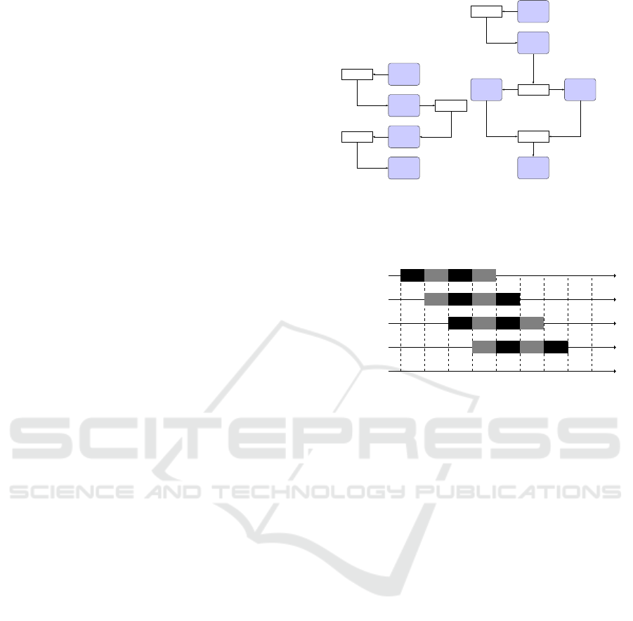
Figure 2: Tree parallelization. The curly arrows represent

threads. The rectangles are terminal leaf nodes.

2.2.3 Parallelization Methods

There are three parallelization methods for MCTS

(i.e., root parallelization, leaf parallelization, and tree

parallelization) that belong to two main categories:

(A) parallelization with an ensemble of trees, and (B)

parallelization with a single shared tree.

The root parallelization method belongs to cate-

gory (A). It creates an ensemble of search trees (i.e.,

one for each thread). The trees are independent of

each other. When the search is over, they are merged,

and the action of the best child of the root is selected.

The leaf parallelization and tree parallelization

methods belong to category (B). In the leaf par-

allelization, the parallel threads perform multiple

PLAYOUT operations from a non-terminal leaf node

of the shared tree. These PLAYOUT operations are in-

dependent of each other, and therefore there is no data

dependency. In tree parallelization, parallel threads

are potentially able to perform different MCTS op-

erations on a same node of the shared tree (Chaslot

et al., 2008a). Figure 2 shows the tree parallelization

where three threads simultaneously perform different

MCTS operations on the tree. This is the topic of our

research.

The existing parallel implementations for tree par-

allelization are based on ILP (Chaslot et al., 2008a;

Enzenberger and M¨uller, 2010; Mirsoleimani et al.,

2015b; Mirsoleimani et al., 2015a). The tasks are

of the type of ILT, and the only dependency that ex-

ists among them is ILD. The potential concurrency is

exploited by assigning a chunk of iterations to sepa-

rate parallel threads and having them work on sepa-

rate processors. Our proposed algorithm allows im-

plementation of tree parallelization based on OLP.

ICAART 2018 - 10th International Conference on Agents and Artiﬁcial Intelligence

616

3 DESIGN OF 3PMCTS

In this section, we describe our proposed method for

parallelizing MCTS. Section 3.1 describes how the

pipeline pattern is applied in MCTS. Section 3.2 pro-

vides the 3PMCTS algorithm.

3.1 Pipeline Pattern for MCTS

Below we describe how the pipeline pattern is used

as a building block in the design of 3PMCTS. Figure

3 shows two types of pipelines for MCTS. The inter-

stage buffers are used to pass information between the

stages. When a stage of the pipeline completes its

computation; it sends a path of nodes from the search

to the next buffer. The subsequent stage picks a path

from the buffer and starts its computation. Here we

introduce two possible types of pipelines for MCTS.

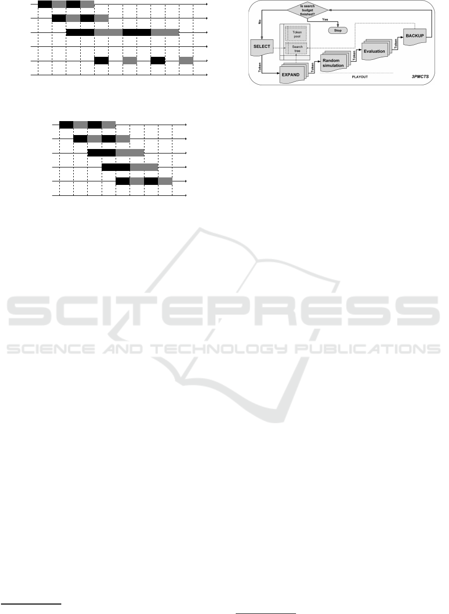
1. Pipeline with sequential stages: Figure 3a shows

a pipeline with sequential stages for MCTS. The

idea is to map each MCTS operation to pipeline

stages so that each stage of the pipeline com-

putes one operation. Figure 4 illustrates how the

pipeline executes the MCTS operations over time.

Let C

represent a multiple-step computation on

path i. C

( j) is the jth step of the computation in

MCTS (i.e., j ∈ {S, E, P, and B}). Initially, the

ﬁrst stage of the pipeline performs C

(S). After

the step has been completed, the second stage of

the pipeline receives the ﬁrst path and computes

(E) while the ﬁrst stage computes the ﬁrst step

of the second path, C

(S). Next, the third stage

computesC

(P), while the second stage computes

(E) and the ﬁrst stage C

(S). Each stage of the

pipeline takes the same amount of time to do its

work, say T. Figure 4 shows that the expected ex-

ecution time for 4 paths in an MCTS pipeline with

four stages is approximately 7 × T. In contrast,

the sequential version takes approximately 16× T

because each of the 4 paths must be processed

one after another. The pipeline pattern works best

if the operations performed by the various stages

of the pipeline are all about equally computation-

ally intensive. If the stages in the pipeline vary in

computational effort, the slowest stage creates a

bottleneck for the aggregate throughput. In other

words, when there are sufﬁcient processors for

each pipeline stage, the speed of a pipeline is

approximately equal to the speed of its slowest

stage. For example, Figure 5 shows the schedul-

ing diagram that occurs when the PLAYOUT stage

takes 2×T units of time while others take T units

of time. Figure 5 shows that the expected execu-

tion time for 4 paths is approximately 11× T.

SelectBuﬀer

Expand

Buﬀer

Playout

Buﬀer

Backup

(a)

SelectBuﬀer

Expand

Buﬀer

Playout Playout

Buﬀer

Backup

(b)

Figure 3: (3a) Flowchart of a pipeline with sequential stages

for MCTS. (3b) Flowchart of a pipeline with parallel stages

for MCTS.

4: PE(B)

3: PE(P)

2: PE(E)

1: PE(S)

4: PE(B)

3: PE(P)

2: PE(E)

1: PE(S)

4: PE(B)

3: PE(P)

2: PE(E)

1: PE(S)

4: PE(B)

3: PE(P)

2: PE(E)

1: PE(S)

4: PE(B)

3: PE(P)

2: PE(E)

1: PE(S)

4: PE(B)

3: PE(P)

2: PE(E)

1: PE(S)

4: PE(B)

3: PE(P)

2: PE(E)

1: PE(S)

4: PE(B)

3: PE(P)

2: PE(E)

1: PE(S)

4: PE(B)

3: PE(P)

2: PE(E)

1: PE(S)

[T]

(S) C

(S)

(E) C

(E)

(P ) C

(P )

(B) C

(B)

Figure 4: Scheduling diagram of a pipeline with sequential

stages for MCTS. The computation for stages are equal.

2. Pipeline with parallel stages: Figure 3b shows a

pipeline for MCTS with two parallel PLAYOUT

stages. Using two PLAYOUT stages in the pipeline

results in an overall speed of approximately T

units of time per path as the number of paths

grows. Figure 6 shows that the MCTS pipeline is

perfectly balanced by using two PLAYOUT stages.

The expected execution time for 4 paths is ap-

proximately 8 × T. Therefore, introducing paral-

lel stages improves the scalability of the MCTS

pipeline.

3.2 Pipeline Construction

The pseudocode of MCTS is shown in Algorithm 1.

Each operation in MCTS constitutes a stage of the

pipeline in 3PMCTS. In contrast to the existing meth-

ods, our 3PMCTS algorithm is based on OLP for

parallelizing MCTS. The pipeline pattern can satisfy

the operation-level dependencies (OLDs) among the

iteration-level tasks (OLTs).

The potential concurrency is also exploited by as-

signing each stage of the pipeline to a separate pro-

cessing element for execution on separate processors.

If the pipeline has only sequential stages then the

speedup is limited to the number of stages.

Pipeline Pattern for Parallel MCTS

617

5: PE(B)

4: PE(Idle)

3: PE(P)

2: PE(E)

1: PE(S)

5: PE(B)

4: PE(Idle)

3: PE(P)

2: PE(E)

1: PE(S)

5: PE(B)

4: PE(Idle)

3: PE(P)

2: PE(E)

1: PE(S)

5: PE(B)

4: PE(Idle)

3: PE(P)

2: PE(E)

1: PE(S)

5: PE(B)

4: PE(Idle)

3: PE(P)

2: PE(E)

1: PE(S)

5: PE(B)

4: PE(Idle)

3: PE(P)

2: PE(E)

1: PE(S)

5: PE(B)

4: PE(Idle)

3: PE(P)

2: PE(E)

1: PE(S)

5: PE(B)

4: PE(Idle)

3: PE(P)

2: PE(E)

1: PE(S)

5: PE(B)

4: PE(Idle)

3: PE(P)

2: PE(E)

1: PE(S)

5: PE(B)

4: PE(Idle)

3: PE(P)

2: PE(E)

1: PE(S)

5: PE(B)

4: PE(Idle)

3: PE(P)

2: PE(E)

1: PE(S)

5: PE(B)

4: PE(Idle)

3: PE(P)

2: PE(E)

1: PE(S)

[T]

(S) C

(S)

(E) C

(E)

(P ) C

(P )

(B) C

(B)

Figure 5: Scheduling diagram of a pipeline with sequential

stages for MCTS. The computation for stages are not equal.

5:PE(B)

4:PE(P)

3:PE(P)

2:PE(E)

1:PE(S)

5:PE(B)

4:PE(P)

3:PE(P)

2:PE(E)

1:PE(S)

5:PE(B)

4:PE(P)

3:PE(P)

2:PE(E)

1:PE(S)

5:PE(B)

4:PE(P)

3:PE(P)

2:PE(E)

1:PE(S)

5:PE(B)

4:PE(P)

3:PE(P)

2:PE(E)

1:PE(S)

5:PE(B)

4:PE(P)

3:PE(P)

2:PE(E)

1:PE(S)

5:PE(B)

4:PE(P)

3:PE(P)

2:PE(E)

1:PE(S)

5:PE(B)

4:PE(P)

3:PE(P)

2:PE(E)

1:PE(S)

5:PE(B)

4:PE(P)

3:PE(P)

2:PE(E)

1:PE(S)

[T]

(S) C

(S)

(E) C

(E)

(P ) C

(P )

(P ) C

(P )

(B) C

(B)

Figure 6: Scheduling diagram of a pipeline with parallel

stages for MCTS. Using parallel stages create load balanc-

ing.

However in MCTS, the operations are not equally

computationally intensive, e.g., the PLAYOUT opera-

tion (random simulations plus evaluation of a terminal

state) could be more computationally expensive than

other operations. Therefore, our 3PMCTS algorithm

uses a pipeline with parallel stages. Introducing par-

allel stages makes 3PMCTS more scalable.

Figure 7 depicts one of the possible pipeline con-

structions for 3PMCTS. We split the PLAYOUT op-

eration into two stages to achieve more parallelism

(See Section 2.1). The ﬁve stages run the MCTS op-

erations SELECT, EXPAND, RANDOMSIMULATION,

EVALUATION, and BACKUP, in that order. The

SELECT stage and BACKUP stage are serial. The

three middle stages (EXPAND, RANDOMSIMULA-

TION, and EVALUATION) are parallel and do the most

time-consuming part of the search. A serial stage does

process one token at a time. A parallel stage is able

to process more than one token. Therefore, it needs

more than one in-ﬂight token. A token represents a

path of nodes inside the search tree during the search.

The pipeline depicted in Figure 7 is one of the

possible constructions for 3PMCTS. Each of the ﬁve

stages could be either serial or parallel. Therefore,

3PMCTS provides a great level of ﬂexibility. For ex-

ample, a pipeline could have a serial stage for the SE-

LECT operation and a parallel stage for the BACKUP

operation. In our experiments we use this construc-

tion (see Section 6).

This holds when the operations performed by the vari-

ous stages are all about equally computationally intensive.

Figure 7: The 3PMCTS algorithm with a pipeline that

has three parallel stages (i.e., EXPAND, RANDOMSIMULA-

TION, and EVALUATION).

4 IMPLEMENTATION

We have implemented the proposed 3PMCTS al-

gorithm in the ParallelUCT package (Mirsoleimani

et al., 2015a). The ParallelUCT package is an open

source tool for parallelization of the UCT algorithm.

It uses task-level parallelism to implement differ-

ent parallelization methods for MCTS. We have also

used an algorithm called grain-sized control paral-

lel MCTS (GSCPM) to measure the performance of

ILP for MCTS. The GSCPM algorithm creates tasks

based on the fork-join pattern (McCool et al., 2012).

More details about this algorithm can be found in

(Mirsoleimani et al., 2015a). Both 3PMCTS and

GSCPM are implemented by TBB parallel program-

ming library (Reinders, 2007) and they are available

online as part of the ParallelUCT package. In our im-

plementation for 3PMCTS, we can specify the num-

ber of in-ﬂight tokens. This is equal to the number of

tasks for GSCPM algorithm.

5 EXPERIMENTAL SETUP

The performance of 3PMCTS is measured by using a

High Energy Physics (HEP) expression simpliﬁcation

problem (Kuipers et al., 2013; Ruijl et al., 2014). Our

setup follows closely (Kuipers et al., 2013). We dis-

cuss the case study in 5.1, the hardware in 5.2, and the

performance metrics in 5.3.

5.1 Case Study

Our case study is in the ﬁeld of Horner’s rule, which

is an algorithm for polynomial computation that re-

duces the number of multiplications and results in a

computationally efﬁcient form. For a polynomial in

one variable

p(x) = a

+ a

n−1

+ ... + a

, (2)

https://github.com/mirsoleimani/paralleluct/

ICAART 2018 - 10th International Conference on Agents and Artiﬁcial Intelligence

618

the rule simply factors out powers of x. Thus, the

polynomial can be written in the form

p(x) = ((a

x+ a

n−1

)x+ ...)x+ a

. (3)

This representation reduces the number of multipli-

cations to n and has n additions. Therefore, the total

evaluation cost of the polynomial is 2n.

Horner’s rule can be generalized for multivariate

polynomials. Here, Eq. 3 applies on a polynomial

for each variable, treating the other variables as con-

stants. The order of choosing variables may be dif-

ferent, each order of the variables is called a Horner

scheme.

The number of operations can be reduced even

more by performing common subexpression elimi-

nation (CSE) after transforming a polynomial with

Horner’s rule. CSE creates new symbols for each

subexpression that appears twice or more and replaces

them inside the polynomial. Then, the subexpression

has to be computed only once.

We are using the HEP(σ) expression with 15 vari-

ables to study the results of 3PMCTS. The MCTS is

used to ﬁnd an order of the variables that gives efﬁ-

cient Horner schemes (Ruijl et al., 2014). The root

node has n children, with n the number of variables.

The children of other nodes represent the remaining

unchosen variables in the order. Starting at the root

node, a path of nodes (variables) inside the search tree

is selected. The incomplete order is completed with

the remaining variables added randomly (i.e., RAN-

DOMSIMULATION). The complete order is then used

for Horners method followed by CSE to optimize the

expression. The number of operations (i.e., ∆) in this

optimized expression is counted (i.e., EVALUATION).

5.2 Hardware

Our experiments were performed on a dual socket In-

tel machine with 2 Intel Xeon E5-2596v2 CPUs run-

ning at 2.4 GHz. Each CPU has 12 cores, 24 hyper-

threads, and 30 MB L3 cache. Each physical core has

256KB L2 cache. The peak TurboBoost frequency is

3.2 GHz. The machine has 192GB physical memory.

We compiled the code using the Intel C++ compiler

with a -O3 ﬂag.

5.3 Performance Metrics

One important metric related to performance and par-

allelism is speedup. Speedup compares the time for

solving the identical computational problem on one

worker versus that on P workers:

speedup =

. (4)

Figure 8: Playout-speedup as function of the number of

tasks (tokens). Each data point is an average of 21 runs

for a search budget of 8192 playouts. The constant C

0.5. Here a higher value is better.

Where T

is the time of the program with one

worker and T

is the time of the program with P work-

ers. In our results we report the scalability of our par-

allelization as strong scalability which means that the

problem size remains ﬁxed as P varies. The problem

size is the number of playouts (i.e., the search bud-

get) and P is the number of tasks. In the literature this

form of speedup is called playout-speedup (Chaslot

et al., 2008a).

The second important metric is the number of op-

erations in the optimized expression. A lower value

is desirable when higher number of tasks is used.

6 EXPERIMENTAL RESULTS

In this section, the performance of 3PMCTS is mea-

sured. Table 1 shows the sequential time to execute

the speciﬁed number of playouts.

Figure 8 shows the playout-speedup for both

3PMCTS and GSCPM, as a function of the number

of tasks (from 1 to 4096). The search budget for both

algorithms is 8192 playouts. The 3PMCTS algorithm

uses a pipeline with ﬁve stages for MCTS operations.

Four stages are parallel; the SELECT stage is chosen

to be serial (see the end of Section 3.2). A playout-

speedup close to 21 on a 24-core machine is observed

for both algorithms. From our results, we may pro-

visionally conclude that the 3PMCTS algorithm (a)

for 4 to 32 parallel tasks, shows a speedup less than

GSCPM and (b) for 64 to 512 parallel tasks, shows a

better speedup than the GSCPM algorithm (see Figure

8). At the same time, 3PMCTS also allows ﬂexible

control of the parallel or serial execution of MCTS

Table 1: Sequential time in seconds when C

= 0.5.

Processor Num. Playouts Time (s)

CPU 8192 215.72 ± 4.12

Pipeline Pattern for Parallel MCTS

619

(a) 3PMCTS (b) GSCPM (c) Root Parallelization

Figure 9: Number of operations as function of the number of tasks (tokens). Each data point is an average of 21 runs for a

search budget of 8192 playouts. Here a lower value is better.

operations (e.g., the SELECT stage is sequential and

the BACKUP stage is parallel in our case), something

that GSCPM cannot provide.

Figure 9a and 9b show the results of the optimiza-

tion in the number of operations in the ﬁnal expres-

sion for both algorithms. These results show consis-

tency with the ﬁndings in (Kuipers et al., 2013; Ruijl

et al., 2014). From our results, we may arrive at three

conclusions. (1) When MCTS is sequential (i.e., the

number of tasks is 1), for small values of C

, such that

MCTS behaves exploitively, the method gets trapped

in local minima, and the number of operations is high.

For larger values of C

, such that MCTS behaves ex-

ploratively, lower values for the number of operations

is found. (2) When MCTS is parallel, for small num-

bers of tasks (from 2 to 8), it turns out to be good to

choose a high value for the constant C

(e.g., 1) for

both 3PMCTS and GSCPM. With higher numbers of

tasks, a lower value for C

in the range [0.5; 1) seems

suitable for both algorithms. Figure 9c also shows

that 3PMCTS can ﬁnd lower number of operations for

8, 16, and 32 tasks when C

= 0.5. (3) When both al-

gorithms ﬁnd the same number of operations, the one

with higher speedup is better. For instance, the 3PM-

CTS algorithm ﬁnds the same number of operations

compared to GSCPM for 64 tasks, but it has higher

speedup when C

= 0.5. Note that these values hold

for a particular polynomial and that different polyno-

mials give different optimal values forC

and number

of tasks.

A comparison to root parallelization is illustrated

in Figure 9c. Both 3PMCTS and GSCPM belong to

the category of tree parallelization. For C

= 0.01,

root parallelization ﬁnds a lower number of opera-

tions for both 16 and 32 tasks compared to the two

other methods. However, increasing the number of

tasks causes root parallelization to provide a much

higher number of operations. From these results, we

may conclude that root parallelization could also be a

feasible choice in this domain.

Kuipers et al. remarked that tree parallelization

would give a result that is statistically a little bit in-

ferior to a run with sequential MCTS with the same

number of playouts due to the violation of iteration-

level dependency (ILD) that produces search over-

head (Kuipers et al., 2015). It is clear from our results

that the effectiveness of any parallelization method

for MCTS depends heavily on the choice of three

parameters: (1) the C

constant, (2) the number of

playouts, and (3) the number of tasks. If we select

these parameters carefully, it is possible to overcome

the search overhead to some extent. Furthermore, the

3PMCTS algorithm provides the ﬂexibility of man-

aging the execution (serial or parallel) of different

MCTS operations that helps us even more to achieve

this goal.

7 CONCLUSION AND FUTURE

WORK

Monte Carlo Tree Search (MCTS) is a randomized

algorithm that is successful in a wide range of opti-

mization problems. The main loop in MCTS consists

of individual iterations, suggesting that the algorithm

is well suited for parallelization. The existing paral-

lelization methods, e.g., tree parallelization, straight

forwardly fans out the iterations over available cores.

In this paper, a new parallel algorithm based on

the pipeline pattern for MCTS is proposed. The idea

is to break-up the iterations themselves, splitting them

into individual operations, which are then parallelized

in a pipeline. Experiments with an application from

High Energy Physics show that our implementation of

3PMCTS scales well. Scalability is only one issue, al-

though it is an important one. The second issue is the

ﬂexibility of task decomposition in parallelism. These

higher levels of ﬂexibility allow ﬁne-grained manag-

ICAART 2018 - 10th International Conference on Agents and Artiﬁcial Intelligence

620

ing of the execution of operations in MCTS which

provide different pipeline constructions. We consider

the ﬂexibility an even more important characteristic

of 3PMCTS. For future work, we will study the ef-

fectiveness of 3PMCTS with regards to the different

pipeline constructions.

ACKNOWLEDGEMENTS

This work is supported in part by the ERC Advanced

Grant no. 320651, “HEPGAME.”

REFERENCES

Browne, C. B., Powley, E., Whitehouse, D., Lucas, S. M.,

Cowling, P. I., Rohlfshagen, P., Tavener, S., Perez, D.,

Samothrakis, S., and Colton, S. (2012). A Survey of

Monte Carlo Tree Search Methods. Computational

Intelligence and AI in Games, IEEE Transactions on,

4(1):1–43.

Chaslot, G., Winands, M., and van den Herik, J. (2008a).

Parallel Monte-Carlo Tree Search. In the 6th Interna-

tioal Conference on Computers and Games, volume

5131, pages 60–71. Springer Berlin Heidelberg.

Chaslot, G. M. J. B., Winands, M. H. M., van den Herik, J.,

Uiterwijk, J. W. H. M., and Bouzy, B. (2008b). Pro-

gressive strategies for Monte-Carlo tree search. New

Mathematics and Natural Computation, 4(03):343–

357.

Coulom, R. (2006). Efﬁcient Selectivity and Backup Op-

erators in Monte-Carlo Tree Search. In Proceed-

ings of the 5th International Conference on Comput-

ers and Games, volume 4630 of CG’06, pages 72–83.

Springer-Verlag.

Enzenberger, M. and M¨uller, M. (2010). A lock-free mul-

tithreaded Monte-Carlo tree search algorithm. Ad-

vances in Computer Games, 6048:14–20.

Fern, A. and Lewis, P. (2011). Ensemble Monte-Carlo Plan-

ning: An Empirical Study. In ICAPS, pages 58–65.

Goodfellow, I., Bengio, Y., and Courville, A. (2016). Deep

Learning. Adaptive Computation and Machine Learn-

ing Series. MIT Press.

Hassabis, D. and Silver, D. (2017). Alphago’s next move.

Kocsis, L. and Szepesv´ari, C. (2006). Bandit based Monte-

Carlo Planning Levente. In F¨urnkranz, J., Scheffer, T.,

and Spiliopoulou, M., editors, ECML’06 Proceedings

of the 17th European conference on Machine Learn-

ing, volume 4212 of Lecture Notes in Computer Sci-

ence, pages 282–293. Springer Berlin Heidelberg.

Kuipers, J., Plaat, A., Vermaseren, J., and van den Herik, J.

(2013). Improving Multivariate Horner Schemes with

Monte Carlo Tree Search. Computer Physics Commu-

nications, 184(11):2391–2395.

Kuipers, J., Ueda, T., and Vermaseren, J. A. M. (2015).

Code optimization in FORM. Computer Physics Com-

munications, 189(October):1–19.

McCool, M., Reinders, J., and Robison, A. (2012). Struc-

tured Parallel Programming: Patterns for Efﬁcient

Computation. Elsevier.

Mirsoleimani, S. A., Plaat, A., van den Herik, J., and Ver-

maseren, J. (2015a). Parallel Monte Carlo Tree Search

from Multi-core to Many-core Processors. In ISPA

2015 : The 13th IEEE International Symposium on

Parallel and Distributed Processing with Applications

(ISPA), pages 77–83, Helsinki.

Mirsoleimani, S. A., Plaat, A., van den Herik, J., and Ver-

maseren, J. (2015b). Scaling Monte Carlo Tree Search

on Intel Xeon Phi. In Parallel and Distributed Systems

(ICPADS), 2015 20th IEEE International Conference

on, pages 666–673.

Reinders, J. (2007). Intel threading building blocks: out-

ﬁtting C++ for multi-core processor parallelism. ”

O’Reilly Media, Inc.”.

Ruijl, B., Vermaseren, J., Plaat, A., and van den Herik, J.

(2014). Combining Simulated Annealing and Monte

Carlo Tree Search for Expression Simpliﬁcation. Pro-

ceedings of ICAART Conference 2014, 1(1):724–731.

Schaefers, L. and Platzner, M. (2014). Distributed Monte-

Carlo Tree Search : A Novel Technique and its Appli-

cation to Computer Go. IEEE Transactions on Com-

putational Intelligence and AI in Games, 6(3):1–15.

Silver, D., Huang, A., Maddison, C. J., Guez, A., Sifre, L.,

Van Den Driessche, G., Schrittwieser, J., Antonoglou,

I., Panneershelvam, V., Lanctot, M., et al. (2016).

Mastering the game of go with deep neural networks

and tree search. Nature, 529(7587):484–489.

Yoshizoe, K., Kishimoto, A., Kaneko, T., Yoshimoto, H.,

and Ishikawa, Y. (2011). Scalable Distributed Monte-

Carlo Tree Search. In Fourth Annual Symposium on

Combinatorial Search, pages 180–187.

Pipeline Pattern for Parallel MCTS

621