Fast Detection and Removal of Glare in Gray Scale Laparoscopic Images
Nefeli Lamprinou and Emmanouil Z. Psarakis
Department of Computer Engineering & Informatics, University of Patras, Rion Patras, Greece
Keywords:
Image Inpainting, Non-blind Inpainting.
Abstract:
Images captured by laparoscopic cameras, often suffer from glare due to specular reflections from surgical
tools and some tissue surfaces that can disturb the attention of surgeon. In this paper, inspired by their form,
the photometric distortions caused by specular reflections are modeled as the superposition of a smooth and
a pulse shaped curve. Based on this model a new fast technique for the detection and removal of glare in
gray scale laparoscopic images is proposed. The proposed technique, as well as other state of the art image
inpainting algorithms are used in a number of experiments based on artificial and real laparoscopic data, and
the proposed algorithm seems to outperform its rivals.
1 INTRODUCTION
Glare is a source of major problems for automated
image analysis systems, as it destroys all information
in affected pixels, a fact that can introduce artifacts
in feature’s extraction algorithms. Image inpainting
is the process of reconstructing lost or deteriorated
regions in an image (Bertalmio et al., 2000). Many
inpainting techniques have been applied in the field
of the medical imaging in order to remove specular
reflections.
Image inpainting methods can be broadly divided into
the following two categories:
• non-blind inpainting and
• blind inpainting.
In the non-blind inpainting, the regions that need to
be filled-in are provided to the algorithm a priori,
whereas in blind inpainting, no information about the
locations of the corrupted pixels is given and con-
sequently the algorithm must additionally identify
the pixels that require inpainting. The state-of-the-
art non-blind inpainting algorithms can perform very
well on removing text, doodle, or even very large ob-
jects (Bertalmio et al., 2000). Some image denois-
ing methods, after modification, can also be applied
to non-blind image inpainting with state-of-the-art re-
sults (Mairal et al., 2008).
Inpainting techniques tailored to repair the glare
due to specular reflections in laparoscopic images fol-
low. In (Lange, 2005) a feature based approach is
used for the detection of the centers of regions that
have been affected by the glare. In order to discover
the total extent of glare’s regions the use of morpho-
logical operators, adaptive thresholding techniques
and the watershed transform is proposed. (Yang et al.,
2010) use a bilateral filter, guided by the maximum
diffuse chromaticity, as well as a technique for its fast
estimation. In (Meslouhi et al., 2011) a method based
on Dichromatic Reflection Model (Artusi et al., 2011)
and multi-resolution (Ogden et al., 1985) inpainting
techniques is presented. Two real time techniques
based on the contrast weighting and intensity sub-
traction are proposed in (Xi and White, 2011). (Sha-
bat and Averbuch, 2012) propose a matrix completion
technique that uses as regularizers the nuclear or the
spectral norm of the matrix. Finally, in (Marcinczak
and Grigat, 2013) the limited accuracy that can be
achieved by thresholding techniques is demonstrated
and a hybrid scheme based on closed contours and
thresholding is proposed.
Blind inpainting, however, is a much harder prob-
lem. Such a technique based on matrix completion
technique using l
0
norm, is proposed in (Yan, 2013).
(Queiroz and Ren, 2014) in order to identify the
glare’s regions propose a segmentation method based
on sparse and low rank matrix decomposition tech-
niques using robust PCA.
In this paper, inspired by their form, the photo-
metric distortions caused by specular reflections are
modeled as the superposition of a smooth and a pulse
shaped curve. Based on this model a new fast tech-
nique for the detection and removal of glare in gray
scale laparoscopic images is proposed.
206
Lamprinou, N. and Psarakis, E.
Fast Detection and Removal of Glare in Gray Scale Laparoscopic Images.
DOI: 10.5220/0006654202060212
In Proceedings of the 13th International Joint Conference on Computer Vision, Imaging and Computer Graphics Theory and Applications (VISIGRAPP 2018) - Volume 4: VISAPP, pages
206-212
ISBN: 978-989-758-290-5
Copyright © 2018 by SCITEPRESS – Science and Technology Publications, Lda. All rights reserved

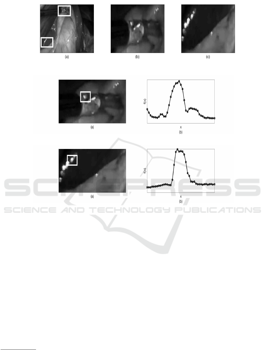
Figure 1: (a): Laparoscopic images with specular reflections due to (b): the surgical tool and (c): the biological tissue (please
see text).
Figure 2: (a): Glare in a laparoscopic image due to the surgical tool. (b): A specific line of the squared region shown in (a).
Figure 3: (a): Glare in a laparoscopic image due to the biological tissue. (b): A specific line of the squared region shown in
(a).
2 SPECULAR REFLECTIONS
AND GLARE
As it was already mentioned, specular reflections cre-
ate strong photometric distortions in laparoscopic im-
ages. Their number, strength as well as shape, are
strongly depended on biological surface angle, cam-
era’s light angle, viewing angle as well as the surgical
tools when they are on the camera’s field of view (see
Figure 1). It is clear that all these photometrically dis-
torted parts of laparoscopic images should be properly
repaired in order to facilitate the tasks of the surgeon.
To this end let us zoom into two lines of the glares
shown in Figure 2 and 3 due to surgical tool and the
biological tissue respectively. Based on these figures
1
we are going to adopt a simple model that can be used
1
It is clear that deconvolving the image line by an appro-
priate kernel which should be strongly related to the PSF of
the gray scale laparoscopic camera, will make our proposi-
tion stronger.
for the description for the aforementioned distortions.
Let f (x) be an image line having K specular re-
flections of width W
k
= x
k+1
−x
k
, k = 0, 1,··· , K −1
each. Then, the following model for the image profile
is considered:
f (x) = f
c
(x) +
K−1
∑
k=0
α
k

u(x −x
k
) −u(x −x
k+1
)

(1)
where f
c
(x) the continuous component of the image,
α
k
, k = 0, 1, ··· , K −1 the K positive heights of the
specular reflections and u(x) the step function.
By taking into account the following weak equal-
ity u
(1)
(x) = δ(x) where δ(x) the distribution delta of
Dirac, the following relation holds:
f
(1)
(x) = f
(1)
c
(x) +
K−1
∑
k=0
α
k

δ(x −x
k
) −δ(x −x
k+1
)

.
(2)
Having defined the specular reflections model, our
goal now is to develop an appropriate technique to
solve the associated estimation problem.
Fast Detection and Removal of Glare in Gray Scale Laparoscopic Images
207

Given the image line profile f (x), let us consider
that the points x
k
, k = 0, 1, ··· , K −1 have been de-
tected and thus they are known. Then, for each pair
(x
k
, x
k+1
), of the aforementioned points, the follow-
ing equations must hold:
f (x
k
) = f
c
(x
k
) + α
k
(3)
f
(1)
(x
k
) = f
(1)
c
(x
k
) + α
k
(4)
f
(1)
(x
−
k
) = f
(1)
c
(x
−
k
) (5)
f (x
k+1
) = f
c
(x
k+1
) + α
k
(6)
f
(1)
(x
k+1
) = f
(1)
c
(x
k+1
) −α
k
(7)
f
(1)
(x
+
k+1
) = f
(1)
c
(x
+
k+1
), (8)
where x
−
, x
+
denotes that we are approaching the
point x from left and right respectively. It is clear that
if the derivative of f (x) is known and based on the
continuity of its continuous counterpart it is an easy
task to properly combine Eqs (3-8) to compute the
desired unknown constant α
k
. However, the afore-
mentioned derivative is unknown and in addition only
a sequence f [n] resulting from the uniform sampling
of the function f (x) is known. Thus, it is necessary
to reformulate the problem at hand in a more prop-
erly stated form where the sequence f [n] instead of
function f (x) is considered to be known. To this end
image’s line model (Eq. (1)) as well as its derivative
(Eq. (2)) are re-expressed into the following discrete
form:
f [n] = f
c
[n] +
K−1
∑
k=0
α
k

u[n −n
k
] −u[n −n
k+1
]

(9)
d
f
[n] = d
f
c
[n] +
K−1
∑
k=0
α
k

δ[n −n
k
] −δ[n −n
k+1
]

,
(10)
where f [.], d
f
[n] are the discrete counterparts of the
functions f (.), f
(1)
(.) and u[.], δ[.] is the step and the
kronecker sequence respectively.
Having defined the discrete counterparts of Eq.
(1) and (2), in the next section we define the discrete
counterparts of Eqs (3-8).
3 THE PROPOSED APPROACH
The discrete counterpart of Eqs (3) and (6) can be
easily defined. However, the discrete counterparts of
the remaining ones are not so straight forward de-
fined. Note that all remaining equations are related
to the derivative of the image line f (x). The use
of derivative-based filters in signal detection prob-
lems has been well documented in the relative liter-
ature. These filters have the ability to remove the
non-stationary component of the signal, while at the
same time preserve abrupt changes, which is highly
desirable in problems of this nature. Note however
that in the case of discrete time signals, there are
three possible approximations of the signal derivative;
namely the forward, the backward, and the forward-
backward first-order difference operators. Although
the third one is the most commonly used in signal de-
tection problems, in this work we propose the use of
the first two, i.e. the forward and the backward differ-
ence operator. Specifically, we propose the use of the
backward difference operator, i.e:
d
f
−
[n] = f [n] − f [n −1] (11)
at the rising edge of the sequence, that is at the point
n
k
, and the use of the f orward difference operator,
i.e.:
d
f
+
[n] = f [n + 1] − f [n] (12)
at the falling one, that is at the point n
k+1
.
We must stress at this point that our choice is
in complete accordance with Eqs (5) and (8) respec-
tively. Concluding, given the pair of points n
k
, n
k+1
the following relations must hold:
d
f
−
[n
k
] = d
f
−
c
[n
k
] + α
k
(13)
d
f
+
[n
k+1
] = d
f
+
c
[n
k+1
] −α
k
, (14)
where d
f
−
c
[.], d
f
+
c
[.]
2
denote the backward and for-
ward difference sequences of the sequence f
c
[.] re-
spectively (a sequence, as it was already mentioned,
resulting from the uniform sampling of continuous
function f
c
(.)). Note that Eqs (13-14) can be ex-
pressed in the form of the following underdetermined
linear system:
Mx
c
k
= b
k
(15)
where
M =

1 0 1
0 1 −1

x
c
k
=

d
f
−
c
[n
k
] d
f
+
c
[n
k+1
] α
k

T
b
k
=

d
f
−
[n
k
] d
f
+
[n
k+1
]

T
with the elements of vector x
c
k
being the quantities
that should be specified.
The above defined system is underdetermined,
thus exhibiting an infinity of solutions, and the goal
is to properly define the excess degrees of freedom.
This can be achieved by using different cost functions
for the specification of different optimum solutions in
2
For space limitation reasons, from now on in some
equations, the brackets from the forward and backward dif-
ference sequences will be omitted.
VISAPP 2018 - International Conference on Computer Vision Theory and Applications
208

R
3
. For instance, the following constrained optimiza-
tion problems can be defined:
(P
l
) : min
x
c
k
∈R
3
||x
c
k
||
l
subject to Mx
c
k
= b
k
, l = 0, 1, 2
and solved for the specification of candidate optimum
solutions. In the next lemma the optimum solution of
optimization problem (P
0
) is specified.
Lemma 1: Consider the optimization problem (P
0
).
Then, its sparsest l
0
optimum solution is the follow-
ing:
x
?
c
k
=


0
d
f
−
[n
k
] + d
f
+
[n
k+1
]
d
f
−
[n
k
]


(16)
or
x
?
c
k
=


d
f
−
[n
k
] + d
f
+
[n
k+1
]
0
−d
f
+
[n
k+1
]


. (17)
Both solutions are optimal and their l
0
norms are
equal to 2.
Proof: The proof is easy and is omitted. 
In the next lemma the optimum solution of opti-
mization problem (P
1
) is specified. As we are going
to see in this case the optimal solution is unique.
Lemma 2: Consider the optimization problem (P
1
).
Then, it attains its l
1
minimum value, i.e.:
||x
?
c
k
||
1
=





|d
f
−
+ d
f
+
|+ d
f
−
, if d
f
+
+ d
f
−
< 0
|d
f
−
+ d
f
+
|−d
f
+
, if d
f
+
+ d
f
−
> 0,
(18)
at:
x
?
c
k
=


























0
d
f
−
[n
k
] + d
f
+
[n
k+1
]
d
f
−
[n
k
]



, if d
f
+
+ d
f
−
< 0



d
f
−
[n
k
] + d
f
+
[n
k+1
]
0
−d
f
+
[n
k+1
]



, if d
f
+
+ d
f
−
> 0.
(19)
In addition, if d
f
+
[n
k+1
] + d
f
−
[n
k
] = 0, then, both so-
lutions described from the branches of Eq. (19) are
optimal.
Proof: The proof is easy and is omitted. 
Finally, the optimization problem (P
2
) can be eas-
ily solved in the least squares sense thus finding the
shortest candidate vector in the space R
3
. The opti-
mum solution is given by the next lemma.
Lemma 3: Consider the constrained optimization
problem (P
2
). Then, it attains its l
2
minimum value:
||x
?
c
k
||
2
=
r
2
3
(d
2
f
−
+ d
2
f
+
+ d
f
−
d
f
+
) (20)
at:
x
?
c
k
=
1
3


2d
f
−
[n
k
] + d
f
+
[n
k+1
]
d
f
−
[n
k
] + 2d
f
+
[n
k+1
]
d
f
−
[n
k
] −d
f
+
[n
k+1
]


(21)
Proof: The proof is easy and is omitted. 
We must stress at this point that since by definition
d
f
−
[n
k
], as the backward difference of the sequence
defined in Eq. (11), is positive while d
f
+
[n
k+1
], as its
forward counterpart, is negative, all optimal solutions
guaranty that the optimum value of α
k
is positive, as
it should be. However, the minimization of either the
l
l
, l = 0, 1, 2 norm does not seem to have any physical
meaning. On the contrary, the l
l
, l = 0, 1, 2 minimiza-
tion of the related elements with the differences of the
smooth counterpart of the sequence, is both attractive
and has physical meaning.
To this end, let us define the following vectors:
x
c
(α
k
) =
h
d
f
−
c
[n
k
] d
f
+
c
[n
k+1
]
i
T
(22)
i = [−1 1]
T
, (23)
and rewrite the underdetermined system (15) as fol-
lows:
x
c
(α
k
) = b
k
+ α
k
i (24)
where vector x
c
(α
k
) is parameterized by glare’s
height α
k
.
Our goal is now to specify the parameter α
k
of the
underdetermined system (24) by solving the follow-
ing constrained optimization problems:
(P
0
l
) : min
α
k
∈R
||x
c
(α
k
)||
l
s. to x
c
(α
k
) = b
k
+ α
k
i, l = 0, 1,2.
It is evident that the optimum solutions of prob-
lems (P
0
l
), l = 0, 1 coincide with that of (P
l
), l = 0, 1.
However, the solution of problem (P
0
2
) does not coin-
cide with the solution of (P
2
). Specifically, the fol-
lowing lemma can be proved.
Lemma 4: The optimum solution of the constrained
optimization problem (P
2
)
0
is attained at:
α
?
k
=
d
f
−
[n
k
] −d
f
+
[n
k+1
]
2
, (25)
with
x
c
(α
k
)[1] = x
c
(α
k
)[2] =
d
f
−
[n
k
] + d
f
+
[n
k+1
]
2
. (26)
This in turn, ensures the shortest Euclidean solution,
that is:
||x
c
(α
?
k
)||
2
=
|d
f
−
[n
k
] + d
f
+
[n
k+1
]|
√
2
. (27)
Proof: The proof is easy. From Eq. (20) the following
relation holds:
||x
c
(α
k
)||
2
2
= 2α
2
k
+ 2 < x
k
, i > α
k
+ ||x
k
||
2
2
, (28)
Fast Detection and Removal of Glare in Gray Scale Laparoscopic Images
209

where < y, z >, ||y||
2
denotes the inner product of the
vectors y and z and the euclidean length of the vector
y respectively. The quadratic expressed by the right
hand side of (25) achieves its minimum value for the
value of α
k
of (24).
This value is definitely positive since by definition
d
f
−
[n
k
] as the backward difference of the sequence
defined in Eq. (11) is positive while d
f
+
[n
k+1
] as
its forward counterpart, is negative. Thus, the quan-
tity defined by (24) is positive and this concludes the
proof of the lemma. 
In the next section we evaluate the performance of
the proposed technique.
4 EXPERIMENTAL RESULTS
In this section we are going to apply the proposed
alignment technique by conducting a number of ex-
periments. In addition, we will compare its perfor-
mance in terms of the achieved alignment error, as
well as its complexity against the methods proposed
in (Shabat and Averbuch, 2012).
4.1 Artificially Distorted 1-D Signals
In this experiment we are going to apply the proposed
technique on artificially distorted 1-D signals. In Fig-
ure 4.(c) such a distorted signal, resulting from the
superposition of the smooth signal (see Fig. 4.(a)):
f
c
[n] = cos(
5π
3
n
1
2
+
π
8
n
1
3
)
and the specular glare (see Fig. 4.(b)):
s[n] = 17(u[n −100] −u[n −125])
respectively, is shown. In addition, its difference
sequence d
f
[n] that can be used for the detection
of glare’s edges x
1
, x
2
, is shown in Figure 4.(d).
The repaired signals obtained from the application of
Lemma 2 and 4 respectively, are shown in Fig. 4.(e)
and 4.(f) respectively. It is clear from this figure that
the optimal solution of the optimization problem de-
fined by Lemma 4 outperforms its rival resulting to a
smoother reconstructed signal profile.
4.2 Real Laparoscopic Images
In this section we are going to apply the proposed
technique in a large number of laparoscopic images
and compare it against the techniques presented in
(Shabat and Averbuch, 2012). Both approaches be-
long to the non-blind inpainting techniques thus re-
quiring the support where the intensity of the image
is known to be given as input. More specifically,
they constitute varieties of matrix completion tech-
nique regularized by the nuclear and the spectral norm
of the matrix respectively. For a given matrix A the
aforementioned norms are defined as:
||A||
?
= trace

√
A
T
A

||A||
2
= max
x
||Ax||
2
||x||
2
= σ
max
(A),
where σ
max
(A) denotes the maximum singular value
of matrix A.
To this end we apply the proposed technique as
well as its rivals in 10K successive frames, each of
size 360 ×640, of the cholecystectomy surgery video.
The results we obtained from the application of the ri-
vals to the specific image frame shown in Figure 5.(a)
are shown in Figures 6, 7 and 8 respectively. From
these figures, and in particular from the zoomed in fig-
ures, seems that the proposed technique outperforms
its rivals since it results in smother, although not per-
fectly, repaired images.That was the case in all the ex-
periments we have conducted. The mean complexity
of the proposed algorithm is 2.2 secs and is error free
in the glare free regions of the image. The mean com-
plexity of its rivals, as well as the achieved MSE in
the known regions of the frames, for different values
of Tolerance for the completion matrix based tech-
niques, are contained in Tables 1 and 2 respectively.
From the contents of these tables, it is clear that the
proposed technique outperforms its rivals. Finally we
must stress at this point that the code of the spectral
norm based completion matrix technique, uses mex
file and this is the reason why it is faster than the nu-
clear norm based one.
Table 1: Performance of the Nuclear based Completion Ma-
trix Technique.
Tolerance 10
−1
10
−3
10
−5
10
−7
10
−9
Time (sec) 2.52 2.12 5.60 13.77 40.12
Mean Error 10
−1
10
−3
10
−5
10
−7
0
Table 2: Performance of the Spectral based Completion Ma-
trix Technique.
Tolerance 10
−1
10
−3
10
−5
10
−7
10
−9
Time (sec) 2.45 2.84 3.32 3.92 5.00
Mean Error 10
−1
0 0 0 0
5 CONCLUSIONS
The proposed technique was applied in a number of
experiments and its superiority over other state of the
VISAPP 2018 - International Conference on Computer Vision Theory and Applications
210

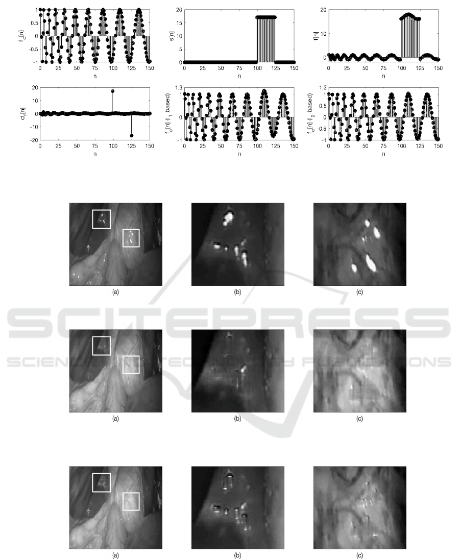
Figure 4: (c): An artificially distorted 1-D signal, resulting from the superposition of (a): the ”smooth” signal, (b): the
specular glare (α = 17) and (d): its discrete difference sequence d
f
[n]. The estimated ”smooth” counterpart of signals, after
the application of (f): Lemma 2 and (e): Lemma 4 on the contaminated signal (c).
Figure 5: (a): An image extracted from a cholecystectomy surgery video containing photometric distortions due to specular
reflections. (b), (c): Zoomed in of the squared regions shown in (a) with specular distortions in details.
Figure 6: The repaired image resulting from the application of the proposed technique on the specularly distorted image
shown in Figure 5.(a). (b), (c): Zoomed in of the squared regions shown in (a) with specular distortions in details (please see
text).
Figure 7: The repaired image resulting from the application of the Nuclear norm based Completion Matrix technique on the
specularly distorted image shown in Figure 5.(a). (b), (c): Zoomed in of the squared regions shown in (a) with specular
distortions in details (please see text).
art image alignment algorithms was indicated. How-
ever, the quality of the repaired images, even from the
proposed method is not perfect, and this, as well as, its
applicability to different kind of images is currently
under investigation. This will make possible the com-
parison of the proposed technique against more re-
Fast Detection and Removal of Glare in Gray Scale Laparoscopic Images
211

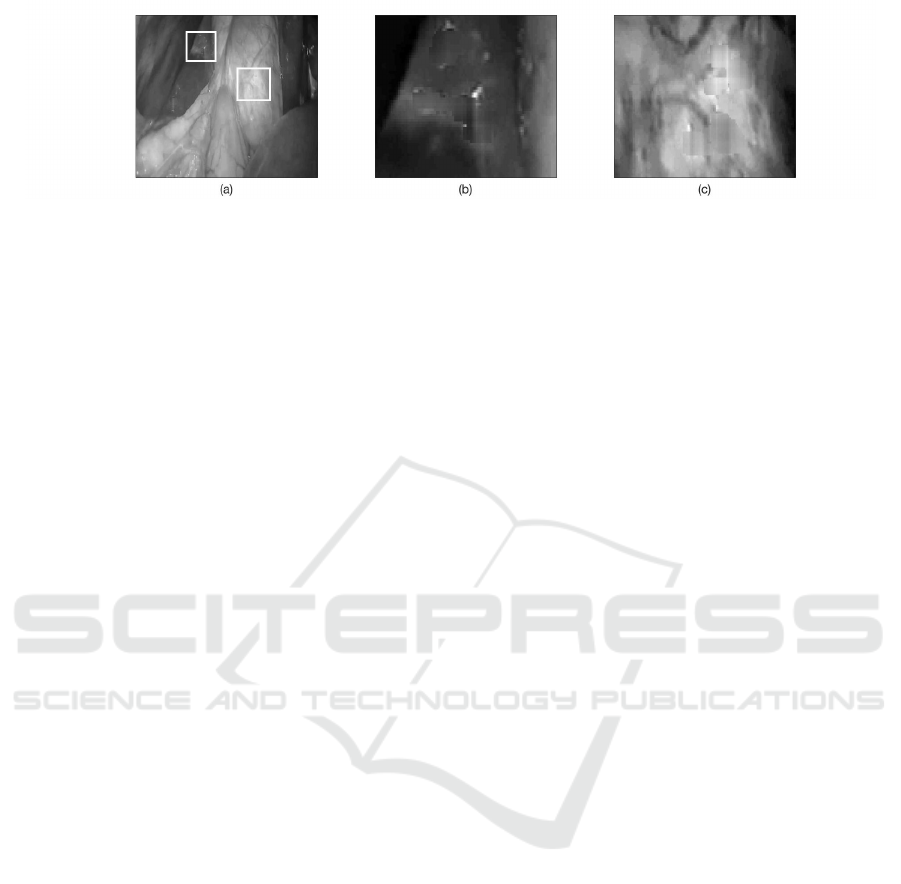
Figure 8: The repaired image resulting from the application of the Spectral norm based Completion Matrix technique on
the specularly distorted image shown in Figure 5.(a). (b), (c): Zoomed in of the squared regions shown in (a) with specular
distortions in details (please see text).
cent based on deep learning image inpainting meth-
ods. Moreover, in order to ensure the applicability of
the proposed algorithm in real time video processing,
the reduction of its mean complexity constitutes a vi-
tal issue that is also under investigation.
ACKNOWLEDGEMENTS
This research was supported by the State Scholar-
ships Foundation (IKY) under contract 23384 −2016
on behalf of the program “Research Projects for
Excellence- IKY/Siemens”.
REFERENCES
Artusi, A., Banterle, F., and Chetverikov, D. (2011). A
survey of specularity removal methods. Computer
Graphics Forum, 30(8):2208–2230.
Bertalmio, M., Sapiro, G., Caselles, V., and Ballester, C.
(2000). Image inpainting. Proceedings of the 27th
Annual Conference on Computer Graphics and Inter-
active Techniques, pages 417–424.
Lange, H. (2005). Automatic glare removal in reflectance
imagery of the uterine cervix. In Proceedings Medical
Imaging, volume 5747.
Mairal, J., Elad, M., and Sapiro, G. (2008). Sparse represen-
tation for color image restoration. IEEE Transactions
on Image Processing, 17(1):53–69.
Marcinczak, J. M. and Grigat, R. R. (2013). Closed con-
tour specular reflection segmentation in laparoscopic
images. International Journal of Biomedical Imaging,
Hindawi Publishing Corporation, 2013:1–6.
Meslouhi, O. E., Kardouchi, M., Allali, H., Gadi, T., and
Benkaddour, Y. A. (2011). Automatic detection and
inpainting of specular reflections for colposcopic im-
ages. Central European Journal of Computer Science,
1(3):341–354.
Ogden, J. M., Adelson, E. H., Bergen, J. R., and Burt, P. J.
(1985). Pyramid-based computer graphics. RCA En-
gineer, 30(5):4–15.
Queiroz, F. and Ren, T. I. (2014). Automatic segmentation
of specular reflections for endoscopic images based
on sparse and low-rank decomposition. In SIBGRAPI
Conference on Graphics, Patterns and Images.
Shabat, G. and Averbuch, A. (2012). Interest zone matrix
approximation. Electronic Journal of Linear Algebra,
23(1):678–702.
Xi, E. A. W. and White, P. (2011). Methods for remov-
ing glare in digital endoscope images. Surgical En-
doscopy, 25:3898–3905.
Yan, M. (2013). Restoration of images corrupted by im-
pulse noise using blind inpainting and l
0
norm. SIAM
Journal of Imaging Sciences, 6(3):1227–1245.
Yang, Q., Wang, S., and Ahuja, N. (2010). Real-time specu-
lar highlight removal using bilateral filtering. In Euro-
pean Conference on Computer Vision (ECCV), pages
87–100.
VISAPP 2018 - International Conference on Computer Vision Theory and Applications
212