Transferring Information Across Medical Images of Different Modalities

Jakub Nalepa

1,2

, Piotr Mokry

, Janusz Szymanek

and Michael P. Hayball

1,3,4

Future Processing, Gliwice, Poland

Silesian University of Technology, Gliwice, Poland

Feedback PLC, Cambridge, U.K.

Cambridge Computed Imaging, Cambridge, U.K.

Keywords:

Multimodal Analysis, ROI Transfer, DICOM.

Abstract:

Multimodal analysis plays a pivotal role in medical imaging and has been recognized as an established tool

in clinical diagnosis. This joint investigation allows for extracting various bits of information from images of

different modalities, which can complement each other to provide a comprehensive view to the patient case.

Since those images may be acquired using different protocols, their synchronization and transferring infor-

mation, e.g., regions of interest (ROIs) between them is not trivial. In this paper, we derive the formulas for

mapping ROIs between different modalities and show a real-life PET/CT example of such image processing.

1 INTRODUCTION

Multimodal image information is useful not only for

visualization, analysis and interpretation of the ima-

ges, but also for undertaking multicenter clinical con-

sultations which allow for improving patient care

by designing better therapy and follow-up strategies.

Therefore, such approaches become common practice

in clinical and pre-clinical imaging, and they are a

very active research topic worldwide. In practical

scenarios, combining the structural (anatomical) in-

formation with the functional information is of the

biggest value. The ultimate goal of multimodal ima-

ging is to maximize the diagnostic (and very often

prognostic for several combinations (Greulich and

Sechtem, 2015)) value of differently acquired images

which may not be fully exploited otherwise.

There are numerous approaches for multimodal

analysis that couple different image modalities in both

side-by-side and fusion modes (Greulich and Sech-

tem, 2015). In the latter techniques, the images re-

quire further processing—they need to be registered,

due to potential misplacement caused by patient brea-

thing or motion (Deregnaucourt et al., 2016). Clinical

cases have shown that single-photon emission compu-

ted tomography/computed tomography (SPECT/CT)

and positron emission tomography/computed tomo-

graphy (PET/CT) are the established diagnostic tools

for radiologists (Pichler et al., 2008). An important

downside of CT imaging is a signiﬁcant radiation

dose that affects the patient, and the limited soft tissue

contrast provided by CT. Therefore, coupling magne-

tic resonance imaging (MRI) with PET (in PET/MRI

systems) is being intensively developed—such sys-

tems can deliver morphologic, functional and mole-

cular information simultaneously (Estorch and Car-

rio, 2013; Vandenberghe and Marsden, 2015). The

current challenges in the multimodal imaging have

been summarized in several surveys and reviews (Es-

torch and Carrio, 2013; Mart

ı-Bonmat

ı et al., 2010;

Sui et al., 2012).

In this paper, we focus on the side-by-side analysis

of multimodal images. We derive formulas for trans-

ferring information between images, using only the

acquisition protocol information available in DICOM

(Digital Imaging and Communications in Medicine),

being a standard for exchanging medical image data.

The formulas can be easily applied to images of any

modalities in order to transfer annotated regions of

interests (ROIs) between them. This ROI transfer is

very useful in techniques for automated segmentation

and analysis of multimodal medical images—as alre-

ady mentioned, the structural information can be en-

hanced by the functional information in search of va-

rious tissues of interest (Nalepa et al., 2016).

Section 2 deﬁnes the prerequisites which are used

in Section 3 to derive formulas utilized for transfer-

ring ROIs across different modalities. In Sect. 4, we

show a real-life example of transferring information

between PET and CT. Section 5 concludes the paper.

526

Nalepa, J., Mokry, P., Szymanek, J. and Hayball, M.

Transferring Information Across Medical Images of Different Modalities.

DOI: 10.5220/0006653305260533

In Proceedings of the 7th International Conference on Pattern Recognition Applications and Methods (ICPRAM 2018), pages 526-533

ISBN: 978-989-758-276-9

2 DEFINITIONS AND USEFUL

EQUALITIES

In this section, we gather the prerequisites, and derive

and prove useful equalities that will become handy in

Section 3—they will be exploited to retrieve the equa-

tions for mapping ROIs between images of different

modalities.

Deﬁnition 1. Consider the following orthonormal vectors:

= (F

) and

= (F

)

where

| = 1, |

| = 1 ⇒

⇒ F

+ F

= F

+ F

= 1 (1)

◦

= F

+ F

= 0 (2)

Additionally, let us introduce

~n = (n

) =

. (3)

Expanding Eq. 3, we obtain:

~n =















· F

− F

· F

− F

· F

− F

· F





where

j and

k are versors. According to this deﬁnition, we have |~n| = 1,

◦~n = 0, and

◦~n = 0. For

and ~n, the following theorem is true:

Theorem 1.

×~n and

=~n ×

Proof.

×~n =



Eq. 1

====





− F

) − F

− F

)

− F

) − F

− F

)

− F

) − F

− F

)









− F

+ F

− F

+ F

− F

+ F









+ F

) − F

+ F

)

+ F

) − F

+ F

)

+ F

) − F

+ F

)





Eq. 2

====





+ F

) + F

+ F

) + F

+ F

) + F





Eq. 1

====











The second proof is analogous.

Remark 1. According to Theorem 1, the following formulas hold:







= F

− F

= F

− F

= F

− F

(4)







= F

− F

= F

− F

= F

− F

(5)

Transferring Information Across Medical Images of Different Modalities

527

Additionally, we can proof the following:

Theorem 2. The inverse matrix of

R =







0 0 0 1







constructed from

and ~n can be expressed as:

−1







0 0 0 1







Proof. The determinant of the R matrix is:

detR = F

− F

) + F

− F

) + F

− F

)

Eq. 4

====

= F

+ F

Eq. 1

==== 1 (6)

Let us calculate the cofactor matrix R







− F

0 0 0 detR







Eq. 4, 5, 1

=======







0 0 0 1







Therefore—by the deﬁnition of the inverse matrix—we have:

−1

detR

)







0 0 0 1







. (7)

3 TRANSFERRING ROIS ACROSS

MODALITIES

In this section, we derive the formulas for transfer-

ring ROIs across different modalities. We exploit

the expressions presented and proven in the previous

section, as well as the image information which can

be extracted from each DICOM ﬁle

. The derived

equations are independent from the underlying mo-

dality, and can be easily applied to process any pair of

modalities side-by-side.

Let



















∆r F

∆c n

∆s S

∆r F

∆c n

∆s S

∆r F

∆c n

∆s S

0 0 0 1



















= A













, (8)

where:

• P

xyz

—Coordinates of the voxel (c,r) in the image plane (in mm).

• S

xyz

—Image position (0020,0032 DICOM attribute). It is the location from the origin (in mm).

For more details see: http://nipy.org/nibabel/dicom/dicom orientation.html; last access date: Oct. 9, 2017.

ICPRAM 2018 - 7th International Conference on Pattern Recognition Applications and Methods

528

• F

:,1

, F

:,2

—Column (Y ) and row (X) direction cosine of the image orientation (0020,0037 DICOM attribute).

These vectors are normal, and F

:,1

◦ F

:,2

= 0.

• r—Row index to the image plane. The ﬁrst row index is zero.

• ∆r, where ∆r 6= 0—Row pixel resolution of the pixel spacing (0028,0030 DICOM attribute) (in mm).

• c—Column index to the image plane. The ﬁrst column index is zero.

• ∆c, where ∆c 6= 0—Column pixel resolution of the pixel spacing (0028,0030 DICOM attribute) (in mm).

• s—Slice index to the slice plane. The ﬁrst slice index is zero.

• ∆s, where ∆s 6= 0—Spacing between the consecutive slices (in mm).

• n

, where i ∈ {1,2,3}—Vector orthogonal to F

:,1

and F

:,2

Taking into account the deﬁnition of ~n (see Eq. 3 and Def. 1, especially Eq. 1), the determinant of the A matrix

becomes:

detA =



∆r F

∆c n

∆s S

∆r F

∆c n

∆s S

∆r F

∆c n

∆s S

0 0 0 1



= ∆r∆c∆s ·



0 0 0 1



Eq. 6

==== ∆r∆c∆s · 1 6= 0.

Consider the following decomposition of the A matrix into the translation, rotation and scaling matrices:

A = T · R · S, (9)

(10)

where

T =







1 0 0 S

0 1 0 S

0 0 1 S

0 0 0 1







,R =







0 0 0 1







,S =







∆r 0 0 0

0 ∆c 0 0

0 0 ∆s 0

0 0 0 1







. (11)

Let us multiply the right side of Eq. 9:

T ·R · S =







1 0 0 S

0 1 0 S

0 0 1 S

0 0 0 1













0 0 0 1













∆r 0 0 0

0 ∆c 0 0

0 0 ∆s 0

0 0 0 1













1 0 0 S

0 1 0 S

0 0 1 S

0 0 0 1













∆r F

∆c n

∆s 0

∆r F

∆c n

∆s 0

∆r F

∆c n

∆s 0

0 0 0 1













∆r F

∆c n

∆s S

∆r F

∆c n

∆s S

∆r F

∆c n

∆s S

0 0 0 1







= A

Such decomposition helps ﬁnd the inverse matrix of A.

Remark 2. Since detA = ∆r∆c∆s 6= 0, T , R and S are invertible (Theorem 2):

−1







1 0 0 −S

0 1 0 −S

0 0 1 −S

0 0 0 1







−1







0 0 0 1







−1







∆r

0 0 0

∆c

0 0

∆s

0 0 0 1







. (12)

Transferring Information Across Medical Images of Different Modalities

529

In order to transfer ROIs across images, P

xyz

values (in Eq. 8) should be the same for both of them (the d and

s subscripts denote the destination and source image, respectively). Therefore, we get:













= A

·V







∆r

∆c

∆s

∆r

∆c

∆s

∆r

∆c

∆s

0 0 0 1































= A

·V







∆r

∆c

∆s

∆r

∆c

∆s

∆r

∆c

∆s

0 0 0 1



















Then:

· R

· S

· V

= T

· R

· S

· V

→

−1

(13)

−1

· T

· R

· S

· V

= R

· S

· V

→

−1

(14)

−1

· T

−1

· T

· R

· S

· V

= S

· V

→

−1

(15)

−1

· R

−1

· T

−1

· T

· R

· S

· V

= V

(16)

−1

· R

−1

) · (T

−1

· A

) · V

= V

(17)

= A

−1

· A

· V

(18)

Let us continue with Eq. 17:

−1

· R

−1

) =







∆r

0 0 0

∆c

0 0

∆s

0 0 0 1













0 0 0 1







⇒

−1

· R

−1

) =







∆r

∆c

∆s

0 0 0 1







(19)

−1

· A

) =







1 0 0 −S

0 1 0 −S

0 0 1 −S

0 0 0 1













∆r

∆c

∆s

∆r

∆c

∆s

∆r

∆c

∆s

0 0 0 1







⇒

−1

· A

) =







∆r

∆c

∆s

− S

∆r

∆c

∆s

− S

∆r

∆c

∆s

− S

0 0 0 1







. (20)

Let us introduce the vector

D, given as:

D =













− S





(21)

and:

−1

· A

) =







∆r

∆c

∆s

∆r

∆c

∆s

∆r

∆c

∆s

0 0 0 1







(22)

ICPRAM 2018 - 7th International Conference on Pattern Recognition Applications and Methods

530

Combining Eq. 19 and Eq. 20, we obtain:

−1

· A







∆r

∆c

∆s

0 0 0 1













∆r

∆c

∆s

∆r

∆c

∆s

∆r

∆c

∆s

0 0 0 1













∆r

+ F

)

∆c

∆r

+ F

)

∆r

∆c

+ F

)

∆c

+ F

)

∆r

∆s

+ n

)

∆c

∆s

+ n

)

0 0

∆s

∆r

+ F

)

∆r

+ F

)

∆s

∆c

+ F

)

∆c

+ F

)

∆s

+ n

)

∆s

+ n

)

0 1







From the deﬁnition of the dot product, we get:

−1

· A







∆r

(

◦

)

∆c

∆r

(

◦

)

∆s

∆r

(

◦ ~n

)

∆r

◦

∆r

∆c

(

◦

)

∆c

(

◦

)

∆s

∆c

(

◦ ~n

)

∆c

◦

∆r

∆s

(~n

◦

)

∆c

∆s

(~n

◦

)

∆s

(~n

◦ ~n

)

∆s

(~n

◦

0 0 0 1







Using Eq. 18 gives:













= A

−1

· A

· V







∆r

(

◦

)

∆c

∆r

(

◦

)

∆s

∆r

(

◦ ~n

)

∆r

◦

∆r

∆c

(

◦

)

∆c

(

◦

)

∆s

∆c

(

◦ ~n

)

∆c

(

◦

∆r

∆s

(~n

◦

)

∆c

∆s

(~n

◦

)

∆s

(~n

◦ ~n

)

∆s

(~n

◦

0 0 0 1



















Finally, we have:











∆r



∆r

(

◦

) + ∆c

(

◦

) + ∆s

(

◦ ~n

) + (

◦



∆c



∆r

(

◦

) + ∆c

(

◦

) + ∆s

(

◦ ~n

) + (

◦



∆s



∆r

(~n

◦

) + ∆c

(~n

◦

) + ∆s

(~n

◦ ~n

) + (~n

◦



(23)

Transferring Information Across Medical Images of Different Modalities

531

Eq. 23 can be used to transfer the information

(e.g., ROIs) across images.

4 CASE STUDY: PET/CT LUNG

SEGMENTATION AND

ANALYSIS

Lung cancer accounts for 12.7% of the world’s total

cancer incidence, and the PET/CT imaging plays a pi-

votal role in its diagnosis, staging and treatment, as it

provides both anatomical and functional information

about the patient. Therefore, automated PET/CT seg-

mentation and analysis techniques attracted research

attention and they are actively being developed (Mo-

kri et al., 2012; Zhao et al., 2015). In our very recent

work (Nalepa et al., 2016), we proposed an automa-

ted approach for PET/CT image analysis which does

not require any user intervention. The experimental

study (44 patients, age: 68.7 ± 10.3 years, 32 males

who underwent FDG-PET/CT using GE Discovery;

the clinical information was available for 42 patients:

I: 1, II: 9, III: 28, and IV: 4) revealed that our auto-

mated histogram-based texture analysis (Miles et al.,

2013) of ﬁltered images

allowed for predicting sur-

vival (kurtosis, p = .028). Therefore, we showed that

using quantitative techniques (CT texture analysis) in

addition to existing measures, including size, density

and glucose uptake, can enhance the diagnostic efﬁ-

ciency of PET/CT.

Algorithm 1: Hands-free PET/CT analysis algorithm.

1: Identify co-registered CT and PET series;

2: Segment lungs in CT;

3: Segment hot-spots in PET in the lung range;

4: Transfer hot-spot ROIs to CT;

5: Apply texture analysis algorithm in CT;

6: Generate report;

The high-level pseudo-code of our hands-free

PET/CT analysis algorithm is presented in Algo-

rithm 1 (we boldfaced the steps which require trans-

ferring information between modalities). After iden-

tifying the co-registered CT and PET series (line 1),

the CT frames are segmented in search of lungs (their

base and apex). Then, the PET images are processed

(line 3), only in the lung region (between base and

apex). First, a threshold is extracted (40% of the glo-

bal maximum pixel value, as suggested in (Win et al.,

2013)). This threshold is used to identify hot-spots in

We used our TexRAD software for texture analysis:

http://texrad.com/.

PET images (connected regions exceeding this value).

Hot-spots are transferred back to CT using Eq. 23 de-

rived in Section 3 (line 4). In the last step, we ap-

ply the TexRAD algorithm (line 5), and generate a

report (line 6) which is saved for review. TexRAD

is a ﬁltration-histogram approach to texture analysis

which comprises image ﬁltration performed to high-

light image features of a speciﬁed size. This proce-

dure is followed by the histogram analysis for quan-

tiﬁcation of derived features using various measures

(e.g., kurtosis, skewness, standard deviation or en-

tropy). Such texture features were shown to be cor-

related with various clinical parameters (Weiss et al.,

2014; Parikh et al., 2014), not only in oncology (Ra-

dulescu et al., 2014).

Example images generated at the most important

steps of the processing pipeline are shown in Figure 1.

The images are co-registered, and the CT frames are

segmented to ﬁnd lungs (Figure 1a). Additionally, in

our approach the convex hulls of lungs are determined

(those regions are larger compared with the segmen-

ted lungs), since the tumors may be associated with

the lung wall or mediastinum. Then, the lung ROIs

are transferred to PET (using Eq. 23) to ﬁnd the lo-

cation of lungs in PET series, and the hot-spots are

segmented (Figure 1b). Afterwards, the hot-spot ROI

is transferred back to the corresponding CT image (by

location), and it undergoes the texture analysis at vari-

ous spatial frequencies (scales). Finally, the extracted

texture features, along with the ﬁltered images are sa-

ved in reports and can be further investigated. This

PET/CT analysis example shows how to efﬁciently

exploit the information (functional and anatomical)

about the patient exposed by two different modali-

ties. The key part of this analysis is concerned with

the possibility of transferring data (e.g., ROIs) across

the co-registered images, as presented in Section 3.

It is worth mentioning that the lung and hot-spot seg-

mentation algorithms can be easily replaced with new,

perhaps more efﬁcient techniques without impacting

the entire hands-free processing pipeline. For more

details, see (Nalepa et al., 2016).

5 CONCLUSIONS

In this paper, we focused on the side-by-side analysis

of multimodal medical images, and derived formulas

which can be used to transfer information (e.g., ROIs)

across different modalities. Since the formulas are ge-

neric, they can be very easily applied to any pair of co-

registered images. Such multimodal analysis became

crucial in the clinical practice because it enhances the

diagnostic efﬁciency of this kind of imaging by cou-

ICPRAM 2018 - 7th International Conference on Pattern Recognition Applications and Methods

532

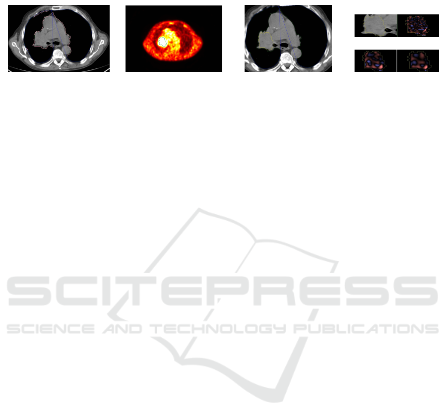
(a) Lungs in CT (b) Hot-spots in PET (c) Transfer (PET→CT) (d) Texture analysis

(i) Original

(ii) Fine

texture

(iii) Medium

texture

(iv) Coarse

texture

Figure 1: Example images generated at the most important steps of the PET/CT analysis: (a) lungs segmented in CT (light

pink ROIs indicate lungs, whereas blue ROIs show their convex hulls), (b) hot-spot segmented in PET, (c) hot-spot transferred

from PET to CT (annotated in yellow), and (d) texture analysis at various scales (ﬁne, medium and coarse) using the TexRAD

algorithm. We boldfaced the steps in which we beneﬁt from transferring the information between two modalities.

pling complementary patient information (e.g., ana-

tomical and functional). It leads to extracting new in-

formation about the patient condition and treatment

response, which would not be revealed if the images

were processed separately.

ACKNOWLEDGEMENTS

This research was supported by the National

Centre for Research and Development under the

Innomed Research and Development Grant No.

POIR.01.02.00-00-0030/15.

REFERENCES

Deregnaucourt, T., Samir, C., and Yao, A.-F. (2016). A

regression model for registering multimodal images.

Procedia Computer Science (MIUA 2016), 90:42 – 47.

Estorch, M. and Carrio, I. (2013). Future challenges of mul-

timodality imaging. In Schober, O. and Riemann, B.,

editors, Mol. Imag. in Onc., pages 403–415, Heidel-

berg. Springer.

Greulich, S. and Sechtem, U. (2015). Multimodality ima-

ging in coronary artery disease – “the more the bet-

ter?”. Cor et Vasa, 57(6):e462 – e469.

Mart

ı-Bonmat

ı, L., Sopena, R., Bartumeus, P., and Sopena,

P. (2010). Multimodality imaging techniques. Con-

trast Media & Molecular Imaging, 5(4):180–189.

Miles, K., Ganeshan, B., and Hayball, M. (2013). CT

texture analysis using the ﬁltration-histogram met-

hod: what do the measurements mean? Canc. Im.,

13(3):400–406.

Mokri, S. S., Saripan, M. I., Marhaban, M. H., and Nordin,

A. J. (2012). Lung segmentation in CT for thoracic

PET-CT registration through visual study. In Proc.

IEEE-EMBS, pages 550–554.

Nalepa, J., Szymanek, J., Mcquaid, S., Endozo, R., Pra-

kash, V., Ganeshan, B., Menys, A., Hayball, M. P.,

Ezhil, V., Bellamy, L., Crawshaw, J., Hall, J., Groves,

A. M., and Nisbet, A. (2016). PET/CT in lung cancer:

An automated imaging tool for decision support. In

Radiological Society of North America 2016 Scienti-

ﬁc Assembly and Annual Meeting, pages 1–2, Chicago

IL, USA. RSNA.

Parikh, J., Selmi, M., Charles-Edwards, G., Glendenning,

J., Ganeshan, B., Verma, H., Mansi, J., Harries, M.,

Tutt, A., and Goh, V. (2014). Changes in primary bre-

ast cancer heterogeneity may augment midtreatment

MR imaging assessment of response to neoadjuvant

chemotherapy. Radiology, 272(1):100–112.

Pichler, B. J., Judenhofer, M. S., and Pfannenberg, C.

(2008). Multimodal imaging approaches: PET/CT

and PET/MRI. In Semmler, W. and Schwaiger, M.,

editors, Molecular Imaging I, pages 109–132, Heidel-

berg. Springer.

Radulescu, E., Ganeshan, B., Shergill, S. S., Medford,

N., Chatwin, C., Young, R. C., and Critchley, H. D.

(2014). Grey-matter texture abnormalities and redu-

ced hippocampal volume are distinguishing features

of schizophrenia. Psychiatry Research: Neuroima-

ging, 223(3):179 – 186.

Sui, J., Adali, T., Yu, Q., Chen, J., and Calhoun, V. D.

(2012). A review of multivariate methods for mul-

timodal fusion of brain data. J. of Neurosc. Met.,

204(1):68 – 81.

Vandenberghe, S. and Marsden, P. K. (2015). PET-MRI:

a review of challenges and solutions in the develop-

ment of integrated multimodality imaging. Physics in

Medicine and Biology, 60(4):R115.

Weiss, G. J., Ganeshan, B., Miles, K. A., Campbell, D. H.,

Cheung, P. Y., Frank, S., and Korn, R. L. (2014).

Noninvasive image texture analysis differentiates k-

ras mutation from pan-wildtype nsclc and is prognos-

tic. PLOS ONE, 9(7):1–9.

Win, T., Miles, K. A., Janes, S. M., Ganeshan, B., Shastry,

M., Endozo, R., Meagher, M., Shortman, R. I., Wan,

S., Kayani, I., Ell, P. J., and Groves, A. M. (2013).

Tumor heterogeneity and permeability as measured on

the ct component of PET/CT predict survival in pa-

tients with non–small cell lung cancer. Clin. Cancer

Res., 19(13):3591–3599.

Zhao, J., Ji, G., Qiang, Y., Han, X., Pei, B., and Shi, Z.

(2015). A new method of detecting pulmonary no-

dules with PET/CT based on an improved watershed

algorithm. PLOS ONE, 10(4):1–15.

Transferring Information Across Medical Images of Different Modalities

533