
Convolutional Neural Networks for Phoneme Recognition
Cornelius Glackin
1
, Julie Wall
2
, Gérard Chollet
1
, Nazim Dugan
1
and Nigel Cannings
1
1
Intelligent Voice Ltd., London, U.K.
2
School of Architecture, Computing and Engineering, University of East London, U.K.
Keywords: Phoneme Recognition, Convolutional Neural Network, TIMIT.
Abstract: This paper presents a novel application of convolutional neural networks to phoneme recognition. The
phonetic transcription of the TIMIT speech corpus is used to label spectrogram segments for training the
convolutional neural network. A window of a fixed size slides over the spectrogram of the TIMIT utterances
and the resulting spectrogram patches are assigned to the appropriate phone class by parsing TIMIT’s phone
transcription. The convolutional neural network is the standard GoogLeNet implementation trained with
stochastic gradient descent with mini batches. After training, phonetic rescoring is performed in the usual way
to map the TIMIT phone set to the smaller standard set. Benchmark results are presented for comparison to
other state-of-the-art approaches. Finally, conclusions and future directions with regard to extending the
approach are discussed.
1 INTRODUCTION
Traditionally, Automatic Speech Recognition (ASR)
involves multiple successive layers of feature
extraction to compress the amount of information
processed from the raw audio so that the training of
the ASR does not take an unreasonably long time.
However, in recent years with increases in
computational speed, the adoption of parallel
computation with General Purpose Graphic
Processing Units (GPGPUs), and advances in neural
networks (the so-called Deep Learning trend), many
researchers are replacing traditional ASR algorithms
with data-driven approaches that simply take the
audio data in its frequency form (e.g. spectrogram)
and process it with a Deep Neural Network (DNN),
or more appropriately, since speech is temporal, a
Recurrent Neural Network (RNN) that can be trained
quickly with GPUs. The RNN then converts the
spectrogram directly to phonetic symbols and in some
cases directly to text (Hannun et al., 2014).
Convolutional Neural Networks (CNNs) present
an interesting alternative to the use of DNNs and
RNNs for ASR. In this paper, we will demonstrate
how the CNN, which is known for state of the art
performance for image processing tasks, can be
adapted for learning the Acoustic Model (AM)
component of an ASR system. The AM model is
responsible for extracting acoustic features from
speech and classifying them to symbol classes.
Specifically, in the CNN Acoustic Model (CNN-AM)
presented in this paper we use spectrograms as input
and phonemes as output classes for training. We will
use the phonetic transcription of the TIMIT corpus as
the ‘ground truth’ for training, validation and testing
the CNN-AM.
2 CNN-BASED ACOUSTIC
MODELLING
A CNN is usually employed for the classification of
static images, see for example (Krizhevsky,
Sutskever and Hinton, 2012). They are inspired by
receptive fields in the mammalian brains which are
formed by neurons in the V1 processing centres of our
cortex responsible for vision; they are also present in
the cochlear nucleus of the auditory processing areas
(Shamma, 2001). The receptive field of a sensory
neuron transforms the firing of that neuron depending
on its spatial input (Paulin, 1998). Usually there is an
inhibitory region surrounding a receptive field which
suppresses any stimulus which is not altered by the
bounds of the receptive field. In this way, receptive
fields behave like feature extractors.
190
Glackin, C., Wall, J., Chollet, G., Dugan, N. and Cannings, N.
Convolutional Neural Networks for Phoneme Recognition.
DOI: 10.5220/0006653001900195
In Proceedings of the 7th International Conference on Pattern Recognition Applications and Methods (ICPRAM 2018), pages 190-195
ISBN: 978-989-758-276-9
Copyright © 2018 by SCITEPRESS – Science and Technology Publications, Lda. All rights reserved
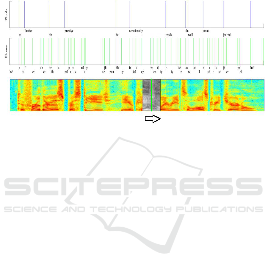
Figure 1: Shows the preparation of the images for GoogLeNet training. A sliding window moves over the 16kHz STFT-
based spectrogram. The sliding window is shown in grayscale, the resulting 256*256 pixel spectrogram patches are placed
into phoneme classes according to the TIMIT transcription for training, validation and testing.
Inspired by the work of Hubel and Wiesel (Hubel
and Wiesel, 1962), Fukushima developed the
Neocognitron network (Fukushima, 1980). Images
are dissected by image processing operations for the
automated extraction of features. These image
processing operations were then formalised by Yann
LeCun to be convolutions; it was LeCun that coined
the term CNN. The most notable example of which
was the LeNet 5 (LeCun et al., 1990) which was used
to learn the MNIST handwritten character data set.
LeNet 5 was the first network to use convolutions and
subsampling or pooling layers.
One of the main strengths of the CNN is that since
Ciresan’s seminal GPU implementation (Ciresan et
al., 2011) in 2011 they are now typically trained in
parallel with a GPU, and in fact are now arguably the
most common type of DNN currently being trained.
One subtlety to note is that the larger the size of the
pooling area, the more information is condensed,
which leads to slim networks that fit more easily into
GPU memory (as they are more linear). However, if
the pooling area is too large, too much information is
thrown away and predictive performance decreases.
The state of the art in CNNs is arguably the
GoogLeNet (Szegedy et al., 2015) which was the
architecture that won the ImageNet competition in
2011 (ILSVRC, 2011).
The main contribution of GoogLeNet is that it
uses inception modules. Convolutions of different
sizes are used within the module and this gives the
network the ability to cope with different types of
features. There are 1x1, 3x3, and 5x5 pixel
convolutions, they are typically an odd number so that
the kernel can be centred on top of the image pixel in
question. In the inception module there are also 1x1
convolutions which reduce the dimension of the
feature vector, ensuring that the number of
parameters to be optimised remains manageable. In
fact, this reduced number of parameters is probably
the principle contribution of the GoogLeNet CNN, it
contains 4 million parameters, whereas its fore-runner
AlexNet (Krizhevsky, Sutskever and Hinton, 2012)
has 60 million parameters to be optimised. The
pooling layer reduces the number of parameters, but
its primary function is to make the network invariant
to feature translation. The concatenation layer
constructs a feature vector for processing by the next
layer.
3 PHONEME RECOGNITION
WITH TIMIT
We used spectrograms to train a CNN to perform
speech recognition. For this, we decided to use the
TIMIT corpus to train the acoustic model (CNN) as it
has accurate phoneme transcription (Garofolo et al.,
1993). The TIMIT speech corpus was designed in
1993 as a speech data resource for acoustic phonetic
studies and has been used extensively for the
development and evaluation of ASR studies. TIMIT
contains broadband recordings of 630 speakers
of eight major dialects of American English, each
Convolutional Neural Networks for Phoneme Recognition
191
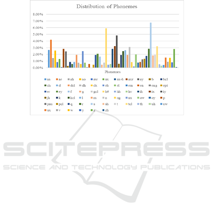
Figure 2: Distribution of phonemes within the TIMIT transcription.
reading ten phonetically rich sentences. The corpus
includes time-aligned orthographic, phonetic and
word transcriptions as well as a 16-bit 16 kHz speech
waveform file for each utterance. TIMIT was
designed to further acoustic-phonetic knowledge and
ASR systems. It was commissioned by DARPA and
worked on by many sites, including Texas
Instruments (TI) and Massachusetts Institute of
Technology (MIT), hence the corpus' name. TIMIT is
the most accurately transcribed speech corpus in
existence as it contains not only transcriptions of the
text but also contains accurate timing of phones. This
is impressive given that the average English speaker
utters 14-15 phones a second. Figure 1 shows a
spectrogram and illustrates the accuracy of the word
and phone transcription for one of TIMIT’s core
training set utterances.
Spectrogram images were generated from the
TIMIT corpus and placed in classes according to
TIMIT’s phone transcription. Spectrograms were
produced for every 160 samples which for 16 kHz
encoded audio corresponds to 10 ms which is the
standard resolution to find all the acoustic features the
audio contains. The contents of the phone ground
truth are parsed and each spectrogram is labelled with
the phone to which its centre falls. Alternatively, one
could have used the centre of the ground truth interval
and calculated the Euclidean distance between the
centre of the phone interval and the window length
but it was decided that this would be making
assumptions about where the phone is centred within
the interval. It would also have required an additional
computationally expensive step in the labelling of the
spectrogram windows.
Figure 1 also illustrates the preparation of the
training, validation and testing data. The figure
illustrates how the phonetic transcription is used to
label the 256x256 greyscale spectrogram patches as
the sliding window passes over each of the TIMIT
utterances. The labelled greyscale patches are sorted
into the directory belonging to each of the 61
phoneme classes for each of the training, validation
and testing sets. In the TIMIT corpus we use the
standard core training setup. We use wide-band or
Short-Term Fourier Transform (STFT) spectrograms,
since we want to align acoustic data with phonetic
symbols with timing that is as accurate as possible.
The FFT component of the spectrogram generation
uses NVIDIA’s cuFFT library for speed. Figure 2
shows the distribution of the phones generated
according to the TIMIT phone transcription in the
training set. For readability purposes, please note that
the bars correspond to the alphabetically ordered
phones in the key below.
As can be seen from the figure, the largest class is
‘s’ and the second largest is ‘h#’ (silence). The latter
occurs at the beginning and end of each TIMIT
utterance. The distribution is unbalanced which of
course makes phoneme recognition by neural
network architectures challenging. The training data
is the standard TIMIT core set, and the standard test
set sub-directories DR1-4 and DR5-8 were used for
ICPRAM 2018 - 7th International Conference on Pattern Recognition Applications and Methods
192
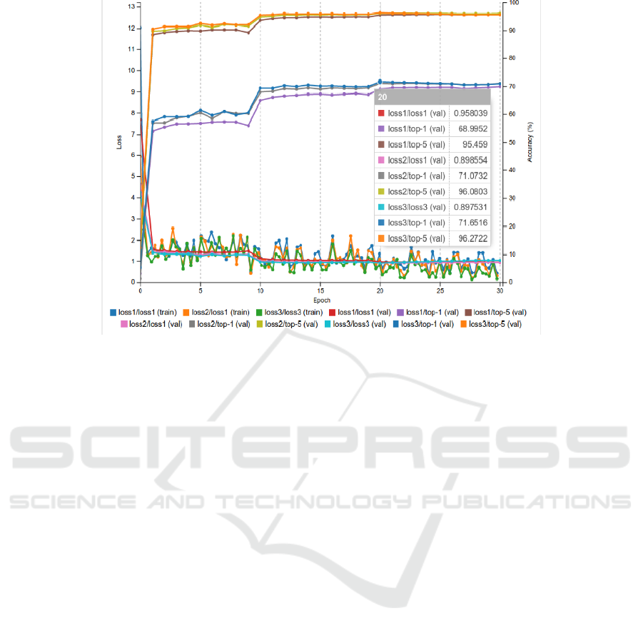
Figure 3: TIMIT stochastic gradient descent training.
validation and testing respectively. This partitioning
resulted in 1,417,588 spectrogram patches in the
training set, as well as 222,789 and 294,101
spectrograms in the validation and testing sets
respectively.
3.1 GoogLeNet Training and
Inferencing
The GoogLeNet implementation was trained with
Stochastic Gradient Descent (SGD). Before the Deep
Learning boom, gradient descent was usually
performed by using the full set of training samples
(full batch) to determine the next update of the
parameters. The problem with this approach is that it
is not parallelizable, and hence cannot by
implemented efficiently on GPU. SGD does away
with this approach by computing the gradient of the
parameters on a single or few (mini batch) training
samples. For large sizes of datasets, such as this one,
SGD performs qualitatively as well as batch methods
but outperforms them in computational time.
A stepped learning rate was used with a 256 data
sample mini batch size, Figure 3 shows the training
accuracy. The network outputs the phone class
prediction at three different points in the network
architecture (loss1, loss2, and loss3). The NVIDIA
DIGITS implementation employed also reports the
top-1 and top-5 predictions for each of those loss
(accuracy) outputs. loss3 (the last network output)
reports the highest accuracy which is 71.65% for
classification of the 61 phones. For top-5 the accuracy
is reported as 96.27%, which means that the correct
phone was listed in the top five output classifications
of the network output, this is interesting because as
mentioned earlier each spectrogram window contains
4 to 5 phones on average, and preliminary tests
confirmed that in the majority of cases the other
phones were indeed correctly being identified.
The network is trained using the training data (1.4
million spectrograms) and it uses the validation set
(approximately 223 thousand spectrograms) to check
training progress. Once this is done there is a separate
testing set (approximately 294 thousand images) that
can be used to test the system, and the standard test
set sub-directories DR1-4 and DR5-8 were used for
validation and testing respectively. The validation set
is used to check the progress of the training of the
network. After each iteration of the training within
which training data has been used to learn the network
weights, the validation data checks that the accuracy
of this latest iteration of the trained system is still
improving. The validation data is kept separate from
the training data and is only used to monitor the
progress of the training, and to stop training if
overfitting occurs. The highest value of the validation
accuracy is used as the final system.
As can be seen in Figure 3, this is at epoch
(iteration) 20, this is the final version of the trained
system. We then use the trained system and perform
inferencing over the test set, Figure 4 shows an
example of the prediction the system makes with a
Convolutional Neural Networks for Phoneme Recognition
193
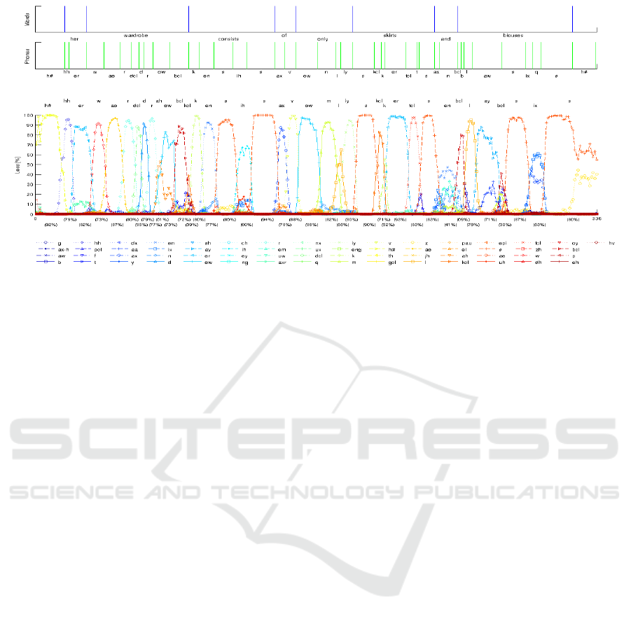
Figure 4: All network outputs for a test utterance.
single sample of this previously unseen test sample.
The output of the inferencing process contains many
duplicates of phones due to the small increments of
the sliding window position.
3.2 Post-processing and Rescoring
Hence, an additional post-processing script was
written to remove the duplicates. It is the convention
in the literature when reporting results for the TIMIT
corpus to re-score the results for a smaller set of
phones (Lopes and Perdigao, 2011). The phoneticians
that scored TIMIT used 61 phone symbols. Many of
the phones in TIMIT are not conventionally used by
other speech recognition systems. For example, there
are phone symbols called closures e.g. pcl, kcl, tcl,
bcl, dcl, and gcl which simply refer to the closing of
the mouth before release of closure resulting in the p,
k, t, b, d, or g phones being uttered respectively. Most
acoustic models map these to the silence symbol ‘h#’.
Post-processing code was written to automatically
remap the output of model inferencing with the new
phone set. The results for the test set were then
generated with the new remapping and the accuracy
increased from 71.65% (shown in Figure 3) to
77.44% after rescoring.
Whilst not quite in excess of the 82.3% result
reported by Alex Graves (Graves, Mohamed and
Hinton, 2013) with bidirectional LSTMs, or the DNN
with stochastic depth (Chen, 2016) which achieved a
competitive accuracy of 80.9%, it is still comparable.
Zhang et al., (Zhang, 2016) is a RNN-CNN hybrid
based on MFCC features. This novel approach uses
conventional MFCC feature extraction with an RNN
layer before a deep CNN structure. The hybrid system
achieved an impressive 82.67% accuracy. It is not
surprising to us that the current state of the art is with
a form of CNN (Tóth, 2015) with an 83.5% test
accuracy. Notably, a team from Microsoft recently
presented a fusion system that achieved the state of
the art accuracy for the Switchboard corpus. Each of
the three ensemble members in the fusion system
used some form of CNN architecture, particularly at
the feature extraction part of the networks. It is
becoming clear that CNNs are demonstrating
superiority over RNNs for acoustic modelling.
Each spectrogram window typically contains 4 or
5 phones per 256 ms window since the average
speaker utters 15 phones per second. The pooling
layers in the CNN-AM provide flexibility in where
the feature under question (phones in this case) can be
within the 256*256 image. This is useful for different
orientations and scales of images in image
classification and is also particularly useful for
phoneme recognition where it is likely there will exist
small errors in the training transcription.
During inferencing (testing), the CNN-AM makes
probabilistic predictions of all the phone classes for
each of the 294,101 test spectrograms. This capability
is provided by the use of softmax nodes at three
successive output stages of the network (Loss 1 to 3).
We carried out some simple graphical analysis of the
output confidences of all the phones, employing
colour coding of the outputs for easier readability of
the results. This graphical analysis is presented in
Figure 4, and as can be seen from the loss-3
(accuracy), the network makes crisp classifications of
usually only a single phone at a time. Given that this
is unseen data, and that the comparison with the
ground truth is good, we are confident that this
ICPRAM 2018 - 7th International Conference on Pattern Recognition Applications and Methods
194

network is an effective way to train an acoustic
model.
4 CONCLUSIONS
We have presented a novel application of CNNs to
phoneme recognition. We have shown how the
TIMIT speech corpus can be used for labelled
spectrogram patches for the CNN-AM training. The
results whilst not surpassing the current state of the
art are encouraging, and the usability and
transparency of the output processing have proved
that CNNs are a very viable way to do speech
recognition. We have also done some initial
experiments with NTIMIT which contains noise from
various telephone networks and as it is telephone
speech it has a narrower frequency range [0, 3.3kHz].
Typically, we have found that NTIMIT results are
around 10% less than for TIMIT. However, we have
found that we are within 1% of the TIMIT networks
performance in our preliminary tests which suggests
that the CNN approach is much more noise robust.
In the near future, we plan to develop strategies to
acquire large volumes of phonetic transcriptions for
training more robust CNN-AM. We are also in the
process of training a sequence-to-sequence language
model to transform the phonetic output to text.
REFERENCES
Chen, D., Zhang, W., Xu, X., & Xing, X., 2016. Deep
networks with stochastic depth for acoustic modelling.
In Signal and Information Processing Association
Annual Summit and Conference (APSIPA), pp. 1-4.
Ciresan, D.C., Meier, U., Masci, J., Gambardella, L.,
Schmidhuber, J., 2011. Flexible, high performance
convolutional neural networks for image classification.
In Int Joint Conf Artificial Intelligence (IJCAI), vol. 22,
no. 1, pp. 1237-1242.
Fukushima, K., 1980. Neocognitron: A self-organizing
neural network model for a mechanism of pattern
recognition unaffected by shift in position. In Biol
Cybern, vol. 36, no. 4, pp. 193-202.
Garofolo, J., Lamel, L., Fisher, W., Fiscus, J., Pallett, D.,
Dahlgren, N., Zue, V., 1993. TIMIT Acoustic-Phonetic
Continuous Speech Corpus LDC93S1. Web Download,
Philadelphia: Linguistic Data Consortium.
Graves, A., Mohamed, A., Hinton, G., 2013. Speech
recognition with deep recurrent neural networks. In
IEEE Int Conf Acoust Speech Signal Process (ICASSP),
pp. 6645-6649.
Hannun, A., Case, C., Casper, J., Catanzaro, B., Diamos,
G., Elsen, E., Prenger, R. et al., 2014. Deep speech:
Scaling up end-to-end speech recognition. In arXiv
preprint arXiv:1412.5567.
Hubel, D.H., Wiesel, T.N., 1962. Receptive fields,
binocular interaction and functional architecture in cat's
visual cortex. In J Physiol (London), vol. 160, pp. 106-
154.
ImageNet Large Scale Visual Recognition Challenge
(ILSVRC), 2011, http://image-net.org/challenges/
LSVRC/2011/index.
Krizhevsky, A., Sutskever, I., Hinton, G.E., 2012. Imagenet
classification with deep convolutional neural networks.
In Adv Neural Inf Process Syst (NIPS), pp. 1097-1105.
LeCun, Y., Boser, B., Denker, J.S., Henderson, D., Howard,
R.E., Hubbard, W., Jackel, L.D., 1990. Handwritten
digit recognition with a back-propagation network. In
Adv Neural Inf Process Syst (NIPS), pp. 396-404.
Lopes, C., Perdigao, F., 2011. Phone recognition on the
TIMIT database. In Speech Technologies/Book 1, pp.
285-302.
NVIDIA DIGITS Interactive Deep Learning GPU Training
System, https://developer.nvidia.com/digits.
Paulin, M.G., 1998. A method for analysing neural
computation using receptive fields in state space. In
Neural Networks, vol. 11, no. 7, pp. 1219-1228.
Szegedy, C., Liu, W., Jia, Y., Sermanet, P., Reed, S.,
Anguelov, D., Erhan, D., Vanhoucke, V., Rabinovich,
A., 2015. Going deeper with convolutions. In IEEE
Conf Computer Vision Pattern Recognition (CVPR),
pp. 1-9.
Shamma, S., 2001. On the role of space and time in auditory
processing. In Trends in Cognitive Sciences, vol. 5, no.
8, pp. 340–348.
Tóth, L., 2015. Phone recognition with hierarchical
convolutional deep maxout networks. In EURASIP
Journal on Audio, Speech, and Music Processing, vol.
1 , pp.1-13.
Xiong, W., Droppo, J., Huang, X., Seide, F., Seltzer, M.,
Stolcke, A., Yu, D. and Zweig, G., 2017. The Microsoft
2016 conversational speech recognition system. In
IEEE Int. Conf. on Acoustics, Speech and Signal
Processing (ICASSP), pp. 5255-5259.
Zhang, Z., Sun, Z., Liu, J., Chen, J., Huo, Z., Zhang, X.,
2016. Deep Recurrent Convolutional Neural Network:
Improving Performance For Speech Recognition, arXiv
1611.07174.
Convolutional Neural Networks for Phoneme Recognition
195
