Performance Visualization for TAU Instrumented Scientiﬁc Workﬂows

Cong Xie

, Wei Xu

, Sungsoo Ha

, Kevin Huck

, Sameer Shende

, Hubertus Van Dam

Kerstin Kleese Van Dam

and Klaus Mueller

Computational Science Initiative, Brookhaven National Laboratory, Upton, New York, U.S.A.

Performance Research Lab, University of Oregon, Eugene, Oregon, U.S.A.

Computer Science Department, Stony Brook University, Stony Brook, New York, U.S.A.

Keywords:

Performance, Visualization, TAU, Scientiﬁc Workﬂow.

Abstract:

In exascale scientiﬁc computing, it is essential to efﬁciently monitor, evaluate and improve performance.

Visualization and especially visual analytics are useful and inevitable techniques in the exascale computing

era to enable such a human-centered experience. In this ongoing work, we present a visual analytics framework

for performance evaluation of scientiﬁc workﬂows. Ultimately, we aim to solve two current challenges: the

capability to deal with workﬂows, and the scalability toward exascale scenario. On the way to achieve these

goals, in this work, we ﬁrst incorporate TAU (Tuning and Analysis Utilities) instrumentation tool and improve

it to accommodate workﬂow measurements. Then we establish a web-based visualization framework, whose

back end handles data storage, query and aggregation, while front end presents the visualization and takes

user interaction. In order to support the scalability, a few level-of-detail mechanisms are developed. Finally, a

chemistry workﬂow use case is adopted to verify our methods.

1 INTRODUCTION

Exascale systems allow applications to execute at un-

precedented scales. With the increased data volume,

the disparity between computation and I/O rates is

more intractable, which leads to ofﬂine data anal-

ysis. Recently, a co-design center focused on on-

line data analysis and reduction at the exascale (CO-

DAR) (I. Foster, 2017) was founded by the Exas-

cale Computing Project (ECP). A new infrastructure

is expected for online data analysis and reduction to

extract and output necessary information and accel-

erate scientiﬁc discovery. On the other hand, sci-

entiﬁc workﬂows are commonly utilized in this sce-

nario to schedule computational processes in paral-

lel and coordinate multiple types of resources for dif-

ferent scientiﬁc applications. Thus, the capability to

capture, monitor, and evaluate the performance of

workﬂows in both ofﬂine and online modes is es-

sential to conﬁrm expected behaviors, discover unex-

pected patterns, ﬁnd bottlenecks, and eventually im-

prove the performance. Since parallel applications

rely on the performance of a number of hardware,

software and application-speciﬁc aspects, the cap-

tured performance evaluation data usually has mul-

tiple dimensions and disjoint attributes. This compli-

cation makes the exploration and understanding ex-

tremely challenging.

Visualization, as an indispensable technique for

big data, has the capability to fuse the multidimen-

sional and heterogeneous evaluation data, provides

corresponding representations for exploration, and

creates effective user interaction and steering. Specif-

ically, performance visualization is the technique fo-

cusing on performance data of heavy computation ap-

plications. The performance data is acquired through

instrumentation of a program, or monitoring system-

wide performance information. It will then be de-

picted to users for the execution evaluation of the

program. There are a number of existing instru-

mentations and/or measurement toolkits such as TAU

(Tuning and Analysis Utilities) (Shende and Mal-

ony, 2006), Score-P (Kn¨upfer et al., 2012) and HPC-

Toolkit (Adhianto et al., 2010). However, none of

these tools can directly handle workﬂow performance

acquisition for either ofﬂine or online modes. This

lack of support from data acquisition end starves the

further development of new performance visualiza-

tion tools for workﬂows.

Therefore, we aim to provide a performance visu-

alization framework dedicated to improving the exe-

cution performance of exascale scientiﬁc workﬂows.

There are three major challenges: 1) the capability

to instrument not only an application, but a scientiﬁc

Xie, C., Xu, W., Ha, S., Huck, K., Shende, S., Dam, H., Dam, K. and Mueller, K.

Performance Visualization for TAU Instrumented Scientiﬁc Workﬂows.

DOI: 10.5220/0006646803330340

In Proceedings of the 13th International Joint Conference on Computer Vision, Imaging and Computer Graphics Theory and Applications (VISIGRAPP 2018) - Volume 3: IVAPP, pages

333-340

ISBN: 978-989-758-289-9

333

workﬂow, 2) the captured performance data itself can

be extremely large, heterogeneous, and collected in a

streaming way, and 3) the cross-platform framework

that handles data management to consume data scale,

provides data aggregation, and supports real-time vi-

sualization, exploration and interaction.

In this paper, on the way to satisfy these require-

ments, we present a proof-of-conceptframework with

data acquisition and handling, as well as a few visual

representation designs for workﬂows. Our framework

is built with ofﬂine analysis use cases, but our design

does not rely on the ofﬂine mechanism, thus is exten-

sible to online. Our contributions are as following:

• An improvement on TAU instrumentation method

to capture parallel workﬂows.

• A web-based framework connecting different

types of performance data into one linked display

with a variety of visual representations.

• A few level-of-detail visual methods enhancing

the data exploration.

The remainder of this paper is structured as fol-

lows: Section 2 summarizes related works, Section 3

discusses our use case, Section 4 introduces the pro-

posed framework, and Section 5 concludes the work.

2 RELATED WORKS

The general purpose of performance evaluation in-

cludes: the global comprehension, problem detection

and diagnosis (Isaacs et al., 2014). Performance visu-

alization is therefore designated to fulﬁll these goals.

At a minimum, the design of the visualization must be

able to show the big picture of the program execution.

When an interesting area is targeted, users must nar-

row down the region and mine more detailed informa-

tion. Moreover, comparative study looking for corre-

lation or dependency must be supported. For problem

detection, abnormal behaviors can be highlighted in

ways that allow users to identify them easily.

Current visualization works can be grouped by

their applications in four contexts: hardware, soft-

ware, tasks and application (Isaacs et al., 2014).

Speciﬁcally, it includes a few types of data: 1) an

event table summarizing the start and end time of all

function calls, 2) the message passing among cores,

3) proﬁling of certain metrics spent in each part of the

code on each computing core, and 4) the call paths.

Therefore, we only summarize the existing works that

are commonly applied to our data types. Other works

such as the visualization for network, system mem-

ory usage, or system logs for multicore clusters can

be found in (Isaacs et al., 2014).

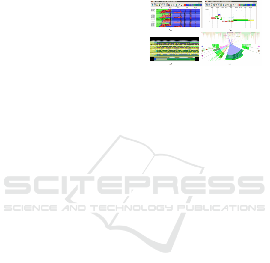
Figure 1: Trace timeline visualization examples: (a) Vampir

timeline showing the execution on all processes (Kn¨upfer

et al., 2008), (b) Vampir timeline for one process with de-

tailed function entry and exit (Kn¨upfer et al., 2008), (c) the

timeline of Jumpshot, and (d) the advanced visualization for

focused thread comparison (Karran et al., 2013).

2.1 Trace Visualization

Tracing measurement libraries record a sequence of

timestamped events such as the entry and exit of func-

tion calls or a region of code, the message passing

among threads, and job initiation of an entire run. A

common practice is to assign the horizontal axis to the

time variable, and the vertical axis to the computation

processes or threads. Different approaches are usually

variations of Gantt charts.

Vampir (Kn¨upfer et al., 2008) and Jump-

shot (Jumpshot, 2014) provide two examples of this

kind of visualization. Generally, overview of the

whole time period is ﬁrst plotted. Then users can

select interested area to reveal more detailed events

happened during the selected period. Different func-

tions or regions of code are colorized, and the black

(yellow for Jumpshot) lines indicate message passing

such as shown in Fig. 1. In addition, advanced visual-

ization tools such as SyncTrace (Karran et al., 2013)

provide a focus view showing multiple threads as sec-

tors of a circle. The relationships between threads

are shown with aggregated edges similar to chord di-

agram. Those tools can only handle small scale data.

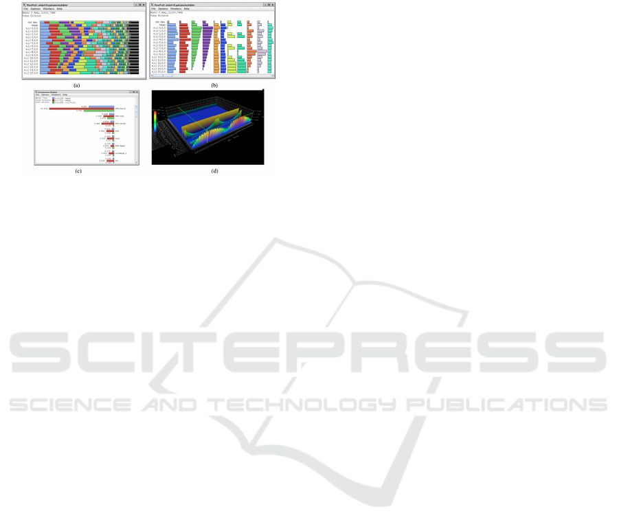
2.2 Proﬁle Visualization

Proﬁling libraries measure the percentage of the met-

ric e.g. time spent in each part of the code. Proﬁle

does not typically include temporal information, but

can quickly identify key bottlenecks in a program.

Stacked bar charts, histogram, and advanced visual-

ization in 3D are commonly used to give a compar-

ative view of the percentage of time or other met-

ric spent for different functions. ParaProf (ParaProf,

2014) is one example of this kind of visualization

as shown in Fig. 2. It also supports the comparison

of certain function calls in different execution runs.

IVAPP 2018 - International Conference on Information Visualization Theory and Applications

334

The functions are color coded and plotted in different

stacking modes. Other statistics can also be plotted

for a selected function over all cores or for a selected

metric correspondingly.

Figure 2: Proﬁle visualization examples: (a) ParaProf

showing the proﬁle of all functions in stacked view (Para-

Prof, 2014), (b) separated view (ParaProf, 2014), (c) the

comparative view of different execution runs (ParaProf,

2014), and (d) the 3D visualization comparing different

metrics (ParaProf, 2014).

2.3 Message Communication

As mentioned in the timeline visualization, message

passing is also important. A straightforward approach

is to draw a line between two functions for each

message, as adopted by Vampir and Jumpshot. On

the other hand, the message communication between

threads or processes can also be summarized in terms

of a matrix, with proper colorization indicating addi-

tional information.

2.4 Limitations

In general, although existing tools are well accepted

by the scientiﬁc community and form as standard ap-

proaches, with tremendous growth in data scale and

computation capability, there are yet some challenges

to solve. Firstly, most approaches are not target-

ing workﬂow executions of many applications. Thus

they lack the capability to illustrate the connection of

workﬂow components and their communication. An-

other issue is the requirement for online evaluation.

This requires online data acquisition, in memory data

processing and visualization. Most existing works are

however designed for ofﬂine analyses. Last but not

least, the acquisition data can be heterogeneous and

should be visualized in a fused and interconnected

way. Our framework is established considering these

aspects.

3 THE USE CASE

NWChemEx (NWChemEX, 2016), as the next gener-

ation of NWChem (Open Source High-Performance

Computational Chemistry), is a scientiﬁc toolkit for

simulating the dynamics of large scale molecular

structures and materials systems on large atomistic

complexes. In our paper, there are two modules:

molecular dynamics (MD) module and the analy-

sis module. Its workﬂow has a structure where the

MD simulation runs in parallel, emitting snapshots

of the protein structure along the trajectory, and con-

currently the data analysis is triggered whenever the

expected data is produced. In our use case, a clas-

sical MD run has 2200 timesteps on 4 nodes while

the corresponding analysis has 1000 timesteps on 1

node. The MD execution took 309.3 seconds wall

clock time in total. We selected the ﬁrst 6.5s to il-

lustrate how our visualization method works.

The major analysis task is for the scientists to

monitor the overall performance of the workﬂow exe-

cution, and explore region of interests in details from

multiple perspectives. In this way, they can apply the

domain knowledge to assess the workﬂow healthiness

and steer the experiment.

4 METHODOLOGY

4.1 TAU Data Acquisition

We adopted TAU instrumentation into the application

code, as well as collected MPI inter-process commu-

nication using the standard PMPI interface (Shende

and Malony, 2006). The post-processed TAU mea-

surements include several types of data: 1) event ta-

ble listing start and end time of all function calls, 2)

the messages passed between processes, 3) proﬁling

of certain metrics spent in each code region on each

computing node/thread, and 4) the call path for each

node/thread.

For a single core execution of a workﬂow com-

ponent, the typical data collected include an event

ﬁle (.edf), a trace ﬁle (.trc) and a proﬁle ﬁle (pro-

ﬁle.*). The ﬁles of independent workﬂow compo-

nents are stored in separate directories. We aggre-

gated the proﬁles and/or traces collected by each com-

ponent with purpose-built post-processing scripts that

generate structured JSON output and merged traces.

Aggregating the proﬁle data is somewhat straightfor-

ward, as the time dimension is collapsed within each

component measurement. However, the trace data in-

cludes detailed communication information between

processes within the component (i.e. MPI messages

Performance Visualization for TAU Instrumented Scientiﬁc Workﬂows

335

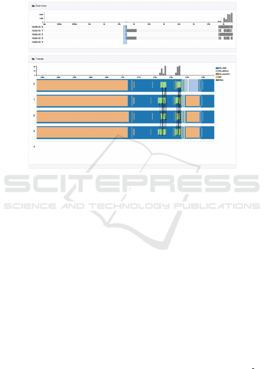
Figure 3: The overview panel (top) and trace detail panel (bottom) of our framework. The overview summarizes the whole

workﬂow execution in a timeline format, where the gray level indicates the density of events (call entry or exit) and the topaxis

shows message counts among nodes/threads. The trace detail expands the detailed function calls and message communication

for the selected nodes. The function calls are color coded according to their functional groups.

from rank m to rank n). Additional post-processing

must be done to remap component ranks within a

global, workﬂow instance rank structure.

Finally, a trace ﬁle and proﬁle ﬁle both in JSON

format were generated and stored into back-end

database. To deal with the scale issue to avoid manag-

ing large ﬁles, instead, separate trace/proﬁle ﬁles can

be generated according to the unique core ID. In our

use case, the size of the single trace ﬁle is 16GB, and

the proﬁle ﬁle is 21MB, both in JSON format.

4.2 The Framework

Considering the analysis tasks, we designed our

framework based on the ”multilevel” visualization

model discussed in (Naser Ezzati-Jivan, 2017) to

store and display the hierarchy of events, with a

proper navigation and exploration mechanism. In de-

tails, we devise a data model including the follow-

ing information: 1) the overall structural description

of the workﬂow, 2) the metadata about the workﬂow,

3) the connected trace events of the entire workﬂow,

and 4) the connected proﬁling of the entire workﬂow.

In order to explore all the above information, we de-

vised and developed a web-based level-of-detail and

multiple-panel visualization framework with a front-

end plotting the data and a back-end performing nec-

essary aggregation and management.

Our front-end visualization includes four major

components: overview, detailed view, node detailed

view, and proﬁle view that together establish an inter-

active analysis platform to visually explore and ana-

lyze the performance of a workﬂow.

4.3 Data Aggregation

Considering the scale of the workﬂows, different vi-

sualization panels must have separate data forms on

the back end to reduce the amount of data sent to front

end. Therefore, for the overviewpanel, we design two

aggregations: 1) the event aggregation by projecting

the events along the timeline into individual time bins,

and 2) the message aggregationby projecting the mes-

sages to histogram along the timeline.

For a function call in the workﬂow, it is rep-

resented by two seperate trace events of func-

tion entry and function exit with the event times-

tamps. For example, the function of “TAU

init”

IVAPP 2018 - International Conference on Information Visualization Theory and Applications

336

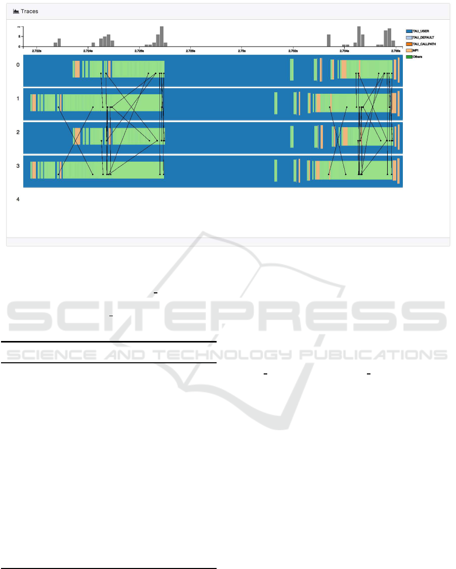
Figure 4: The trace detailed view panel: a coarse level of selected timeline is illustrated. Different transparency can be seen

to enhance function separation when there are many small function calls.

has two events: {“name”:“TAU

init”, “event-

type”:“entry”, “time”:“12305”, “node-id” 3, “thread-

id” 0} and {“name”:“TAU

init”, “event-type”:“exit”,

“time”:“19870594”, “node-id” 3, “thread-id” 0}.

Algorithm 1: Matching entry and exit events of functions

calls.

Require: E = {e} is a list of trace events, t(e) is the

timestamp of e ∈ E. F is the result matched func-

tions. D is the list of the callpath depths of F.

1: function MATCHING(E)

2: sort E by the timestamps

3: s is initialized as an empty stack

4: d ← 0

5: for i ← 1 to |E| do

6: if e

is an entry event then

7: d ← d + 1

8: pop e

into s

9: else

10: d ← d − 1

11: pop e

′

from s

12: push (e

′

, e

) to F, push d to D

13: return F,D

Since the same function can be called and exit

multiple times in one core, pairing the entry and exit

events E into complete functions F is necessary. Fur-

thermore, in these un-matched traces, it is difﬁcult to

ﬁnd the call relationships of different functions. We

proposed Algorithm 1 to pair the events and calculate

the callpath depths D of the functions F. Our algo-

rithm is similar to a balanced parentheses matching

algorithm.

As a result, the trace events E executed

in one core are paired into a set of com-

plete function calls F, (e.g., a function call of

“TAU

init” is {“name”:“TAU init”, “start”:12305,

“end” 19870594, “node-id” 3, “thread-id” 0}). The

paired events are stored and indexed all in a back-end

database, where the detailed view panels can query

directly.

4.4 Overview

Overview shows the summary of the whole workﬂow

execution as in Fig. 3(top). There are two parts: the

trace events, and message counts. The trace events

indicating the start and end time of each function call

are shown as timelines. We use intensity to indicate

the depth of the call path. A darker color represents a

more nested function call. For each node/thread, the

trace events are plotted separately. Above the time-

lines, we also visualized the message counts (sent or

received) in a separate histogram view along the time-

line. For the interaction, it allows the user to select a

time range of interest and see more details in the trace

detailed view panel.

Performance Visualization for TAU Instrumented Scientiﬁc Workﬂows

337

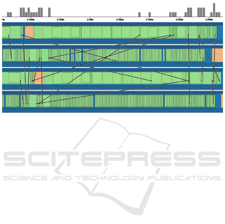
Figure 5: The detailed view panel: a ﬁne level of selected timeline is shown when further zooming in. We enhance the

function separation by adding the borderline to each rectangle. The height of rectangle is adjusted according to its call depth.

4.5 Trace Detailed View

The trace detailed view shows the function calls

and messages in the selected time range as in

Fig. 3(bottom). Each function call is visualized with a

rectangle and its color representing the corresponding

call group. The functions are visualized with nested

rectangles that indicate their depths in the call path.

This fashion is similar to what Jumpshot (Jumpshot,

2014) utilized, but we chose a more compact lay-

out. In this view, users can still zoom in to explore

more details by selecting a smaller time range. This

is shown in Fig. 4.

When there are many short function calls in a

nested call structure, it can be difﬁcult to observe

small events and differentiate each call. Therefore,

we designed three features for that issue:

• First, we use different transparencyto enhance the

visibility of overlapped functions as can be found

in Fig. 4.

• Second, when zooming in, we add the border line

of the rectangle to enhance the separation of dif-

ferent functions, as shown in Fig. 5. They are

color coded according to different call groups.

• Furthermore, in order to enhance the call path

structure, we reduce the height of the rectangle

along a call path. Therefore, a callee function

must have smaller height than a caller function.

As in Fig. 5, where by observing the number of

horizontal lines around a function, users can eas-

ily detect the depth d of the call.

For the message visualization, additionally, we vi-

sualized the message passing (send and receive) be-

tween functions as straight black lines (see Fig. 5).

As being organized in a timeline, the line direction is

ignored since the message is always passing from left

to right. Finally, when hovering over each rectangle,

the detailed function name can be seen in text.

4.6 Node Detail View

In the detailed view, all functions are plotted as nested

rectangles. This design is compact and reﬂects caller-

callee relationship well. However, when there are too

many short function calls one after another, it can be

difﬁcult to track how often and how long each func-

tion is executed. Therefore, we design a node level

detail exploration tool as shown in Fig. 6. This view

is aligned with detailed view panel when user selects

one speciﬁc node to explore. Then the nested rect-

angles are replaced with stacked bar graphs, where

overlapping is avoided. In this new view, the verti-

cal order of each bar graph reﬂects its call path depth.

In Fig. 7, a ﬁne level design with highlighted strokes

around bar graphs further enhances the separation of

functions.

4.7 Proﬁles View

In the Proﬁles view, with the selected metric (time or

counter), we visualize the percentage spent on each

function for each node/thread in stacked bar graphs.

IVAPP 2018 - International Conference on Information Visualization Theory and Applications

338

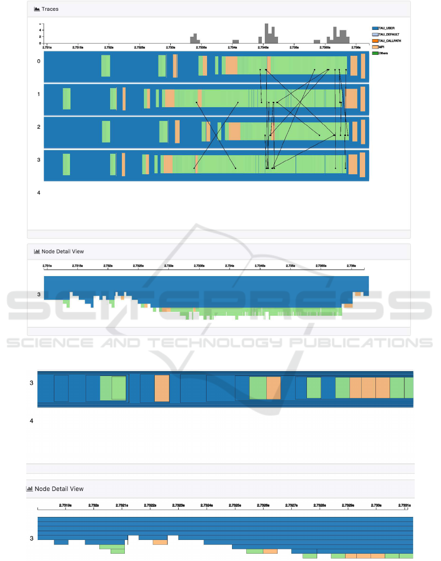
Figure 6: The node detail panel: a coarse level visualization of the selected timeline of node 3 is shown. The trace panel and

the node detail panel are aligned along the time axis, which makes it easy to compare.

Figure 7: The node detail panel: a ﬁne level visualization of the selected timeline is shown when further zooming in; the node

3 is selected, and the borderlines are plotted.

Performance Visualization for TAU Instrumented Scientiﬁc Workﬂows

339

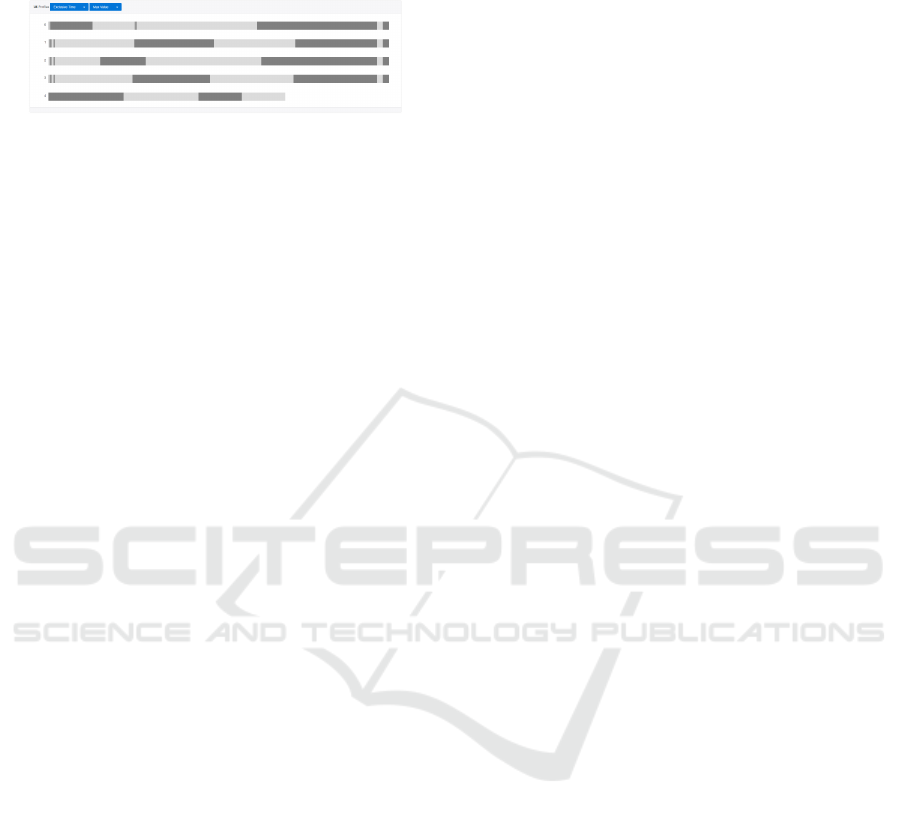
For example, in Fig. 8, we plotted the proﬁle for “ex-

clusive time” metric.

Figure 8: The Proﬁles view: stacked bar graphs to show

proﬁles of nodes with maximum exclusive time metric.

5 CONCLUSION

In this paper, current progress on capturing and vi-

sualizing performance of scientiﬁc workﬂows is pre-

sented. We propose improved workﬂow acquisition,

devise a web-based visualization framework integrat-

ing both trace and proﬁle into one display. In speciﬁc,

we present a few data aggregation methods, propose

the visualization with different levels of details, pro-

vide message communication with both line connec-

tions and message count histograms.

As future work, we have made substantial plans:

1) Back end: more data aggregation mechanism to

enhance scalability; efﬁcient data query and storage

method; 2) Front end: additional levels of detail of

visualization to accommodate aggregation designs in

overview level and trace detail level; workﬂow com-

ponent data ﬂow. We will also work on an extreme-

scale or exascale use case, and conduct more case

studies.

ACKNOWLEDGEMENTS

This research was supported by the Exascale Com-

puting Project (ECP) the Co-design center for Online

Data Analysis and Reduction (CODAR) 17-SC-20-

SC.

REFERENCES

Adhianto, L., Banerjee, S., Fagan, M., Krentel, M., Marin,

G., Mellor-Crummey, J., and Tallent, N. R. (2010).

Hpctoolkit: Tools for performance analysis of opti-

mized parallel programs. volume 22, pages 685–701.

Wiley Online Library.

I. Foster, M. Ainsworth, e. a. (2017). Computing just what

you need: Online data analysis and reduction at ex-

treme scales. Europar.

Isaacs, K. E., Gim´enez, A., Jusuﬁ, I., Gamblin, T., Bhatele,

A., Schulz, M., Hamann, B., and Bremer, P.-T. (2014).

State of the art of performance visualization. In Euro-

graphics/IEEE Conference on Visualization State-of-

the-Art Reports, EuroVis.

Jumpshot (2014). Examining trace ﬁles with jumpshot.

Karran, B., Trumper, J., and Dollner, J. (2013). Sync-

trace: Visual thread-interplay analysis. 2013 First

IEEE Working Conference on Software Visualization

(VISSOFT), 00:1–10.

Kn¨upfer, A., Brunst, H., and et al (2008). The vampir

performance analysis tool-set. Tools for High Perfor-

mance Computing, pages 139–155.

Kn¨upfer, A., R¨ossel, C., Mey, D. a., Biersdorff, S., Di-

ethelm, K., Eschweiler, D., Geimer, M., Gerndt, M.,

Lorenz, D., Malony, A., Nagel, W. E., Oleynik, Y.,

Philippen, P., Saviankou, P., Schmidl, D., Shende, S.,

Tsch¨uter, R., Wagner, M., Wesarg, B., and Wolf, F.

(2012). Score-P: A Joint Performance Measurement

Run-Time Infrastructure for Periscope,Scalasca, TAU,

and Vampir, pages 79–91. SpringerBerlin Heidelberg,

Berlin, Heidelberg.

Naser Ezzati-Jivan, M. R. D. (2017). Multi-scale naviga-

tion of large trace data: A survey. Concurrency and

Computation: Practice and Experience, 29.

NWChemEX (2016). A new generation of nwchem, a high-

performance computational chemistry software pack-

age.

ParaProf (2014). Proﬁle analysis with paraprof.

Shende, S. S. and Malony, A. D. (2006). The tau par-

allel performance system. The International Jour-

nal of High Performance Computing Applications,

20(2):287–311.

IVAPP 2018 - International Conference on Information Visualization Theory and Applications

340