Computing a Multi-location Aircraft Fleet Mix

Slawomir Wesolkowski

, Gregory Patchell

and Akshay Dwarkan

Defence R&D Canada, Ottawa, Canada

Faculty of Mathematics, University of Waterloo, Waterloo, Canada

Faculty of Engineering, University of Ottawa, Ottawa, Canada

Keywords: Genetic Algorithms, Pareto-optimal Solutions, NSGA-II, Multi-objective Optimization.

Abstract: The Canadian Armed Forces periodically examines aircraft, ship or ground vehicle fleets to determine if they

need to reduce, keep the same or increase the number of platforms in their fleets. We adapt previous work on

fleet estimation and multi-objective optimization to compute a Pareto-optimal set of fleets at multiple

locations, taking into account mission scheduling. We apply our model, which uses a genetic algorithm based

on NSGA-II, to a sample of notional scenarios to demonstrate the effectiveness of the approach.

1 INTRODUCTION

A critical decision that military organizations are

faced with is to decide whether to change the number

of platforms (aircraft, ships or ground vehicles) in

their fleets by examining the trade-off space between

operational effectiveness and acquisition cost.

Military procurement costs can be high. For example,

for the acquisition of 63 F-35 fighters, the U.S

Airforce estimated a cost of $10.1 billion (US DOD,

2017), that is, approximately $160 million per

aircraft. These high costs and the need to examine

what capabilities are gained by acquisitions have

motivated the development and application of

optimization and simulation methods to address the

problems of military fleet mix rationalization

(Wojtaszek and Wesolkowski, 2012).

There are many tasks (missions) in the military

such as combat, search and rescue, and transportation

of troops or cargo that require the use of a variety of

platforms. We are concerned with determining the

composition of a new fleet and estimating associated

acquisition costs beyond the current number of

platforms in the fleets. Consequently, we would like

to provide decision makers enough information to

determine whether to add, reduce or keep the same

the number of platforms in the fleets by estimating

how these changes would impact the operational

effectiveness of the missions carried out by the fleets.

Previously developed models such as the

Stochastic Fleet Estimation - Robust (SaFER)

(Wesolkowski and Wojtaszek, 2012) and Training

Device Estimation (TraDE) (Wesolkowski et al.,

2014) have assessed similar procurement problems.

The TraDE model produces a set of training device

configurations (or solutions) that provide trade-offs

between multiple objectives (acquisition cost, travel

cost, operating cost and training time). These

solutions include the number of devices needed, the

device type and the proposed location of the devices,

for a set of tasks to be completed by a number of

troops, while minimizing costs and total training

completion time. Solutions can also be used to

identify redundant devices to reduce annual

maintenance and operating costs.

The SaFER model estimates the size and

composition of aircraft fleets based on mission

requirements and closure times (the maximum time

allowed to complete a mission). SaFER uses a genetic

algorithm (GA) and scheduling heuristics to

effectively order all the missions. These schedules are

then used to compute the minimum or best case core

(steady state) fleet component and surge (transient

state) fleet component requirements, resulting in fleet

mix computations which allow decision makers to

assess the risk of surge requirements for various

aircraft fleet mixes.

The proposed algorithm which is a simplification

and amalgamation of TraDE and SaFER computes a

Pareto-optimal set of vehicle fleets by considering the

current fleet of vehicles at different locations, mission

information, mission scheduling, platform

capabilities, costs and operational effectiveness. The

main advantage of our algorithm and SaFER over

124

Wesolkowski, S., Patchell, G. and Dwarkan, A.

Computing a Multi-location Aircraft Fleet Mix.

DOI: 10.5220/0006646701240131

In Proceedings of the 7th Inter national Conference on Operations Research and Enterprise Systems (ICORES 2018), pages 124-131

ISBN: 978-989-758-285-1

TraDE is that they both incorporate scheduling,

meaning that they take into account the order of

missions that need to be carried out based on the

frequency of mission occurrence and mission priority.

TraDE does not account for specific task completion

times and this may cause scheduling conflicts.

However, TraDE considers the possibility that a

device can be located at various locations. Our

algorithm assumes that a platform cannot move

between locations. SaFER does not take location into

consideration and only uses mission information and

closure times. In addition, TraDE can accommodate

a large number of different locations whereas our

algorithm considers a limited number of locations. On

the other hand, faster results can be obtained with our

algorithm due to its simplicity compared to the TraDE

and SaFER models.

The paper is organized as follows. Section II

describes the problem and the proposed algorithm. In

Section III, we apply the algorithm to an air force

problem using notional data based on information

provided by subject matter experts (SMEs) in the

Royal Canadian Air Force. Finally, in Section IV,

conclusions about the algorithm are made and future

improvements are suggested. Although we have used

an air force problem to demonstrate our model, this

model can be applied to other services (i.e., the navy

and the army).

2 THE ALGORITHM

2.1 Problem Overview

In order to determine the composition of a military

fleet, we need information about the different

missions that the platforms need to complete. A

mission has a particular frequency of occurrence

(how often the mission occurs in a year), a priority

value (“1” being the highest priority) and a closure

time. Closure time refers to the time from the start of

the mission within which the mission has to be

completed. We also consider the various capabilities

of the different platform types and how important

each capability is to each mission. In addition, to

perform a given capability at a specific level of

effectiveness (low, medium or high), different

numbers of platforms are needed. Capability scores

(between 0 and 1) were assigned by SMEs to quantify

low, medium or high capability levels.

Cost and operational effectiveness are major

factors in determining our fleet design. For this

problem, we only consider platform capital

acquisition costs and ignore maintenance and

operating costs. Maintenance and operating costs are

of course very important given that a fleet’s cost over

its lifetime may be higher than the acquisition cost.

Future adjustments to this model will allow us to take

them into account. Operational effectiveness depends

on critical/no-fail capabilities in each mission,

mission scheduling, the number of each platform type

required for each mission, and the effectiveness of

each platform for a given capability.

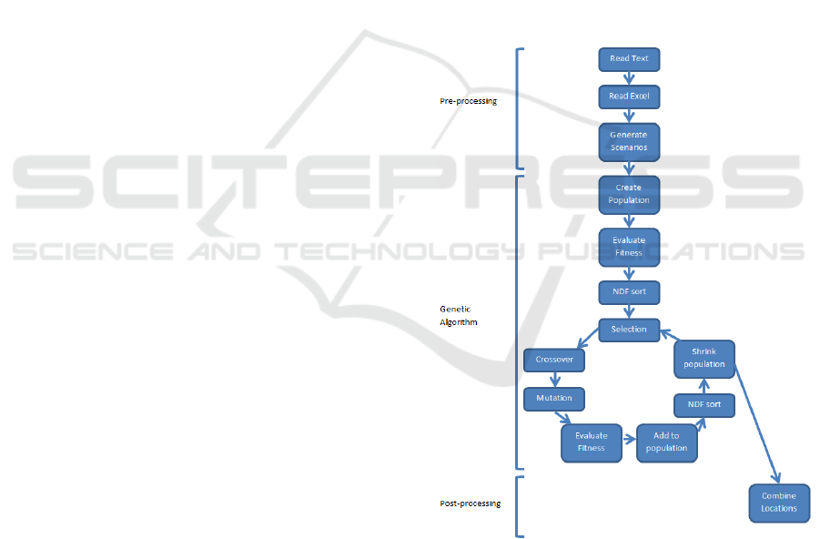
2.2 Algorithm Overview

A multi-objective genetic algorithm is implemented

to simultaneously optimize on two objectives:

acquisition cost and operational effectiveness. Figure

1 shows an overview of the algorithm which consists

of three major parts: pre-processing (data input and

scenario generation), the genetic algorithm, and post-

processing (combining results and generating trade-

off plots).

Figure 1: Algorithm Overview.

First, a set of scenarios is randomly generated for

each location using mission occurrence (how many

instances of each mission occur over a period of 1

year?) and mission duration (how long do these

missions last?) using triangular distributions based on

the data provided in Appendix A. We then apply

NSGA-II (Deb et al., 2002), an elitist GA to each

scenario. In our adaptation of NSGA-II, parent

Computing a Multi-location Aircraft Fleet Mix

125

selection is carried out by first choosing one parent

from the non-dominated front (NDF), and then

choosing the other parent by selecting the fitter of two

candidates via roulette selection. Superior solutions

are obtained with this method compared to the

original NSGA-II crossover which selects both

parents by roulette selection (Deb et al., 2002). The

solutions for the various locations are then

combinatorically combined to create whole fleet

solutions resulting in a large number of fleet mixes

which can respond to a wide variety of multi-location

scenarios.

2.3 Chromosomes

A chromosome (an individual solution) consist of two

parts: the fleet configuration and the mission

schedule. The fleet configuration chromosome part

contains a matrix assigning a number of platforms of

each type to each mission. The bounds on the

configuration are given by minimum fleet and

maximum fleet input (minimum and maximum

number of each platform that can be assigned to a

mission). We also ensure that all capabilities required

for a mission can be assigned at least one platform

type. The schedule chromosome part contains an

ordering of all the mission occurrences (based on

mission frequency). When the schedule is initialized,

the missions with higher priority missions are always

scheduled before lower priority missions.

2.4 Fitness Evaluation

The total number of platforms in the fleet is calculated

by using the fleet configuration and mission ordering

by applying a bin packing algorithm to schedule the

missions (explained in Section II.F). The total number

of platforms corresponds to the number of individual

platforms in each bin (one bin per platform type). The

fitness values (acquisition cost and operational

effectiveness) are then calculated. The non-

dominated front is calculated based on the fitness

values.

2.5 Crossover and Mutation

NSGA-II applies crossover and mutation operators to

the set of solutions (or parents). For the crossover, one

parent is selected from the current non-dominated

front of the parent population. To select the second

parent, two individuals are first randomly chosen

from the entire parent population, and the fittest one

is chosen. We apply a standard crossover operator

which picks, with equal probability, a fleet

configuration from the two parents and assigns it to

the child. When the crossover operator is applied to

the mission schedule, a random swath of consecutive

chromosome values is selected from the first parent

and placed in the same position in the child. These

values are removed from the second parent. The

remaining chromosome values from the second

parent are then used to fill the child chromosome in

order starting from the left.

Each parent’s chromosome can be mutated in two

ways: the fleet configuration and the schedule. The

mutation operator has only one mutation parameter µ,

which is the probability that the fleet configuration is

changed. Mutation of the fleet configuration is carried

out by randomly picking a fleet configuration

between the minimum fleet and maximum fleet. The

schedule is mutated by randomly assigning missions

while preserving priority-based ordering.

Once a set of children has been produced and

mutated, they are combined with the parents to obtain

a set of individuals that is twice the size of the initial

population. Non-dominated front sorting is applied to

this set to select the next generation of population

members. However, if the last front to be placed in

the new population exceeds the remaining space in

the new population (this can occur for the first front

if the number of individuals in the first front exceeds

the population size), the individuals are sorted by

crowding distance to preserve diversity in the solution

set. The crowding distance of an individual is defined

as the sum (over all objectives) of the distance

between its two closest neighbours (Deb et al., 2002).

The process of removing the “most crowded”

individuals from the front is called truncation of the

front.

2.6 Objective Functions

The objective functions are to minimize acquisition

cost and maximize operational effectiveness.

2.6.1 Acquisition Cost

To calculate the total acquisition cost, we need to

compute the total number of platforms in the fleet f,

by scheduling all the missions as follows:

1. Iterate through the mission occurrences using the

mission ordering.

2. Calculate “investment” (i.e., the number of

platforms in configuration * platform cost *

mission duration) that is used to decide which

platforms to schedule first.

3. Number the platforms from highest to lowest in

priority and exclude platforms with an investment

ICORES 2018 - 7th International Conference on Operations Research and Enterprise Systems

126

of 0 (meaning that the platform cannot perform

the mission).

4. Find the platform type with the highest

investment, as it has the highest priority ranking.

5. Schedule the mission occurrence on that platform

type with as many platforms as indicated by the

configuration.

6. Schedule the mission occurrence at the same time

on other platform types with as many platforms as

indicated by the configuration.

7. Add more platforms as needed.

The number of platforms of different type that we

obtain at the end of this process is our fleet. To

calculate the acquisition cost, we then minimize the

following equation:











 





 









where P is the total number of platform types, f

is the

number of platforms of type i in the calculated fleet,

current

is the number of platforms of type i in the

existing (current) fleet and A

is the acquisition cost of

one platform of type i.

2.6.2 Operational Effectiveness

To calculate operational effectiveness, the algorithm

uses the fleet configuration as follows:

1. For each combination of mission, platform type,

and capability, we first consider how many

platforms of that type are used for the mission.

Then, we look at how many platforms are needed

to obtain a low/medium/high score for that

capability on that mission. A score is assigned

based on these two observations.

2. For each combination of mission and capability,

take the maximum platform score.

3. For each combination of mission and capability,

if the capability is no-fail for that mission and the

score is 0, assign the mission a score of 0.

Otherwise, if the capability is required, add the

score for the mission and capability to the mission

score.

4. Normalize the mission scores by how many

capabilities are required for each mission.

5. Take a weighted average of the mission scores

using priority values.

To be clear, this formulation of operational

effectiveness which amalgamates evaluations of very

different capabilities into one score is carried out to

simplify the problem. Once candidate fleets are

identified, a more detailed process examining the

capability trade-offs that come with each solution

would be undertaken.

2.7 Combinations

After running the GA for each location, the solutions

for each location are combined by permuting each

solution from one location with all solutions from the

other locations. The fleets and costs are added

together, and the operational effectiveness scores are

averaged using mission occurrences as weights as

follows:







 



















where L is the total number of locations. oeff

is the

operational effectiveness for one fleet from location i,

and occur

is the total number of mission occurrences

from location i. This allows the final combined

solution to be a set of combined fleets from all

locations of interest. We note that the bounds on the

range of values produced by the function are 0 and 1.

This enables operational effectiveness to be

represented as a percentage of a theoretical maximum

possible operational effectiveness and allows for an

easy way to compare the operational effectiveness of

different fleet mixes.

3 RESULTS

3.1 Experimental Set Up

We consider an air force problem for illustration

purposes. Data on missions, required capabilities for

each mission and related platform capabilities for

various aircraft are notional and are based in part of

information provided by SMEs from the Royal

Canadian Air Force.

Twenty five annual scenarios were tested with

each scenario having a computer runtime of

approximately 3 hours. A scenario is a different

combination of missions (including different mission

durations) at each of the considered base locations.

Due to time limitations for this study, we were only

able to use 25 scenarios at each location resulting in

effectively 15,625 global scenarios. A large number

of scenarios is usually desirable when dealing with

problems with high degrees of uncertainty

(Wesolkowski and Wojtaszek, 2012). We apply

NSGA-II to each scenario at each of the three

locations. We set the mutation rate, µ, to 0.35 and use

a population (individuals) size of 400 iterated over

800 generations.

Computing a Multi-location Aircraft Fleet Mix

127

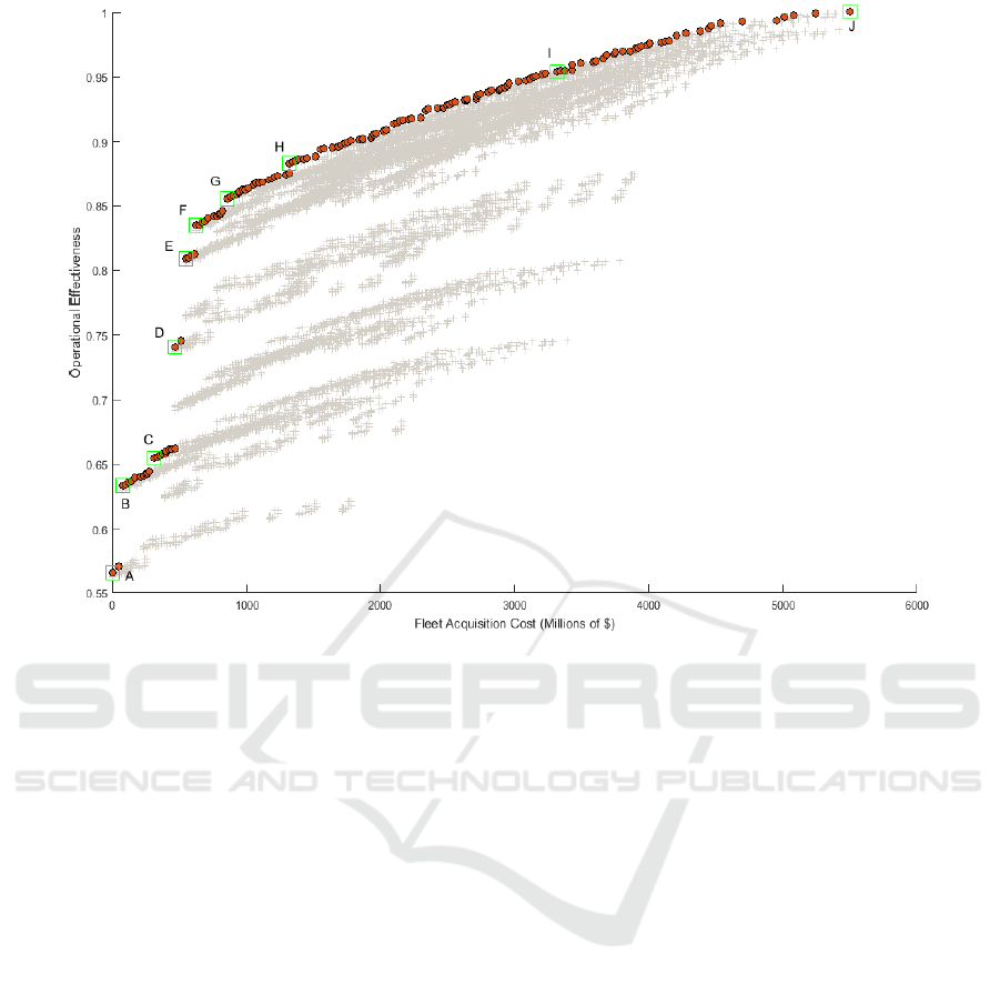
Figure 2: Air fleet mix rationalization trade-off.

The solutions for all scenarios were combined into

a super front, a notional Pareto front, eliminating all

duplicate solutions. The Pareto front, in this case,

represents the solutions to the scenarios which are the

toughest to satisfy (fleet mixes proposed by

dominated solutions would be able to address less

demanding scenarios). Therefore, we use this super

front in our analysis.

3.2 Data

We consider scenarios at each of the three locations:

Loc1, Loc2 and Loc3. Each scenario comprises

various combinations of three missions: M1, M2 and

M3. Four platforms (AC1 to AC4) were considered

for each mission and were assessed on 29 capabilities

(Cap1 to Cap29). Each of the AC1 to AC4 platforms

has an acquisition cost of 22, 87, 78 and 32 million

dollars respectively. We assume that the bases

already had a total of 85 AC1’s, 12 AC2’s, 22 AC3’s

and 12 AC4’s. Low, medium and high capability

scores are set to 0.3, 0.7 and 1 respectively. Finally

we set the Yearly Flying Rate (YFR) per fleet to 4000

hours. Tables 3 to 7 in Appendix A show the notional

data.

3.3 Results and Discussion

Figure 2 shows the trade-off space between

acquisition cost and operational effectiveness. After

running NSGA-II on each location, we

combinatorically combined solutions from each

scenario at one location with solutions from scenarios

run for other locations. In this manner, we obtained a

total of 597,608 unique solutions and 35,120

solutions on the Pareto front for all multi-location

scenarios combined. The selected values in Table 1

are represented by squares in Figure 2. The solutions

on the Pareto front represent fleet mixes which are

able to carry out the most demanding multi-location

scenarios.

Most solutions have a high number of AC1’s and

a low number of AC2’s and AC4’s (see Table 1). We

also observe that as the acquisition cost increases, the

operational effectiveness increases as well.

Furthermore, since all platform types were used in all

the solutions, this particular problem set did not find

any solutions which reduced the number of fleets. The

correlation coefficients between acquisition cost and

operational effectiveness in the Pareto front and the

total set of solutions are 0.8422 and 0.8211

respectively.

ICORES 2018 - 7th International Conference on Operations Research and Enterprise Systems

128

Table 1: Selected points from the Pareto front.

Solution

AC1

AC2

AC3

AC4

Acq. Cost

($M)

Op. Eff

0.5651

0.6337

312

0.6546

468

0.7403

546

0.8089

624

0.8343

858

0.8553

1326

0.8830

3318

0.9591

5499

1.0000

Table 2 shows the correlation coefficients

between each platform type and the objective

function values. It also shows the correlation

coefficients for each pair of platform types. We can

see that AC1, AC2 and AC4 have very weak or

negligible relationships with acquisition cost and

operational effectiveness. AC3 has a very strong

positive relationship with both objective functions.

This would mean that the number of AC3’s plays a

key role in increasing the operational effectiveness of

the fleet and consequently in increasing the

acquisition cost. On the other hand, the relationships

between each pair of platform types are negligible

meaning that their numbers are uncorrelated and

potentially independent of each other.

From $0 – $1000 million, we observe a steep

gradient among the points on the Pareto front (see

Figure 2). This means that for a small increase in

acquisition cost, there is a high gain in operational

effectiveness. We can speak of a “knee” in the Pareto

front at approximately $1000 million, since from

$1000 - $6000 million, the Pareto points have a much

smaller slope, thereby, indicating that for a large

increase in acquisition cost, there is only a small gain

in operational effectiveness.

These observations would play a major role in

deciding a new configuration for the aircraft fleet. For

a military organization on a limited budget, Solution

F (624, 0.8343) consisting of 68 AC1’s, 2 AC2’s, 29

AC3’s and 6 AC4’s could be a cost effective solution

providing operational effectiveness for a

“reasonably” demanding multi-location scenario (see

Figure 2). Deviations from that point can be

considered based on the military organization’s

budget and risk tolerance (higher risk at lower cost

and vice versa). For example, for a lower budget, we

can consider solution E.

Table 2: Correlation coefficients.

AC1

AC2

AC3

AC4

Acq. Cost

-0.167

0.078

0.991

0.198

Op. Eff

-0.104

0.005

0.838

0.047

AC1

1.000

-0.021

0.064

-0.143

AC2

0.021

1.000

-0.125

-0.061

AC3

-0.176

0.064

1.000

0.117

AC4

-0.222

-0.143

0.117

1.000

However if we decrease the acquisition budget too

much, it would cause a drastic loss in operational

effectiveness which might not be acceptable to

decision makers. On the other hand, if the

organization needs an operational effectiveness

higher than 0.8343, they would require a much higher

budget. Increasing operational effectiveness to

0.8830 (Solution H) would increase the acquisition

budget to $1326 million, which is more than double

the $624 million for Solution F.

4 CONCLUSIONS

We have proposed an algorithm to solve a notional air

fleet mix rationalization problem based on a number

of mission scenarios. We applied NSGA-II to solve

this problem. Solutions based on scenarios for three

different locations were combined to create multi-

location fleet mix solutions. These solutions suggest

different fleet mixes to decision makers based on their

risk tolerance and budget. The algorithm is adaptable

to other kinds of fleets such as ground vehicles.

Several improvements could be implemented in

the future. First, maintenance and operational costs

should be considered, as well as training simulations

and required personnel. The algorithm for operational

effectiveness should be investigated in greater detail

to ensure that the values correspond to perceived

capabilities of the resulting fleets. Finally, multi-

scenario experiments should be run multiple times to

assess how well the genetic algorithm converges to a

combined non-dominated front.

Computing a Multi-location Aircraft Fleet Mix

129

REFERENCES

U.S. Department of Defense (US DOD), 2017, Department

of Defense (DoD) Releases Fiscal Year 2017

President’s Budget Proposal. Available online:

https://www.defense.gov/News/News-Releases/News-

Release-View/Article/652687/department-of-defense-

dod-releases-fiscal-year-2017-presidents-budget-

proposal/

Wojtaszek, D., Wesolkowski, S., 2012, Military Fleet Mix

Computation and Analysis. In IEEE Computational

Intelligence Magazine, Vol. 7, No. 3, pp. 53-61, 2012.

Wesolkowski, S., Wojtaszek, D., 2012, Multi-objective

optimization of the fleet mix problem using the SaFER

model, IEEE Congress on Evolutionary Computation.

Wesolkowski, S., Francetic, N., Grant, S.C., 2014, TraDE:

Training device selection via multi-objective

optimization. In IEEE Congress on Evolutionary

Computation (IEEE CEC), pp. 2617-2624.

Deb, K., Pratap, A., Agarwal, S. , and Meyarivan, T., 2002,

A fast and elitist multiobjective genetic algorithm:

NSGA-II. In IEEE Transaction on Evolutionary

Computation, pp. 182–197.

APPENDIX

Table 3 shows the information pertaining to each

mission. A priority value of “1” refers to a mission

with the highest priority. Closure time refers to the

time within which the mission has to be completed.

Frequency shows how often a mission occurs. Table

4 shows the capability requirements for each mission

where “0” means unnecessary, “1” means required

and “2” means no-fail (critical). Tables 5 to 7 show

the number of aircraft needed to perform each

capability at a specific level (low, medium or high).

“0” means the capability is not possible with that

aircraft.

Table 3: Mission information.

Location 1

Mission ID

Mission1

Mission2

Mission3

Priority

Min. Freq

400

Avg. Freq

400

Max. Freq

400

Closure Time Min

120

1000

1400

Closure Time Avg

120

1000

1400

Closure Time

Max

120

1000

1400

Location 2

Priority

Min. Freq

300

Avg. Freq

300

Max. Freq

300

Closure Time Min

120

1000

1400

Closure Time Avg

120

1000

1400

Closure Time

Max

120

1000

1400

Location 3

Priority

Min. Freq

700

Avg. Freq

700

Max. Freq

700

Closure Time Min

120

1000

1400

Closure Time Avg

120

1000

1400

Closure Time

Max

120

1000

1400

Table 4: Mission requirements.

Mission/

Capability

Mission1

Mission2

Mission3

Cap1

Cap2

Cap3

Cap4

Cap5

Cap6

Cap7

Cap8

Cap9

Cap10

Cap11

Cap12

Cap13

Cap14

Cap15

Cap16

Cap17

Cap18

Cap19

Cap20

Cap21

Cap22

Cap23

Cap24

Cap25

Cap26

Cap27

Cap28

Cap29

ICORES 2018 - 7th International Conference on Operations Research and Enterprise Systems

130

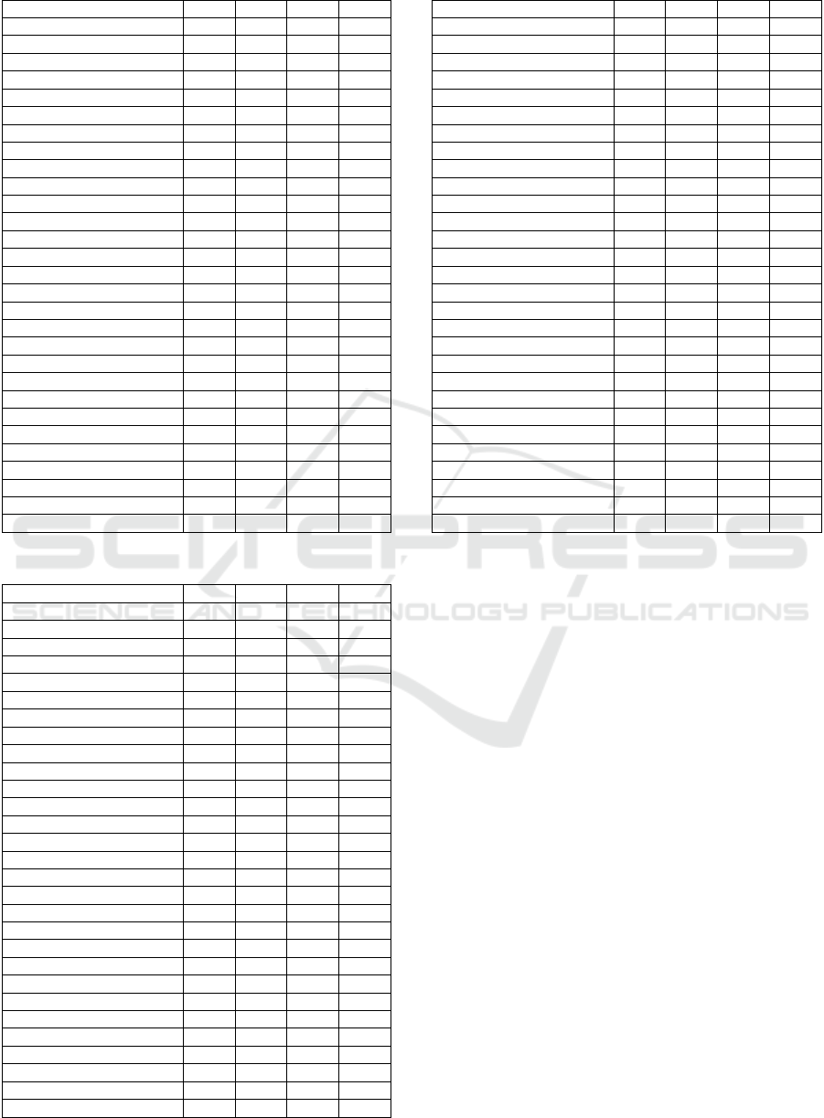
Table 5: Platform capabilities at the low level.

Platform/ Capability

AC1

AC2

AC3

AC4

Cap1

Cap2

Cap3

Cap4

Cap5

Cap6

Cap7

Cap8

Cap9

Cap10

Cap11

Cap12

Cap13

Cap14

Cap15

Cap16

Cap17

Cap18

Cap19

Cap20

Cap21

Cap22

Cap23

Cap24

Cap25

Cap26

Cap27

Cap28

Cap29

Table 6: Platform capabilities at the medium level.

Platform/ Capability

AC1

AC2

AC3

AC4

Cap1

Cap2

Cap3

Cap4

Cap5

Cap6

Cap7

Cap8

Cap9

Cap10

Cap11

Cap12

Cap13

Cap14

Cap15

Cap16

Cap17

Cap18

Cap19

Cap20

Cap21

Cap22

Cap23

Cap24

Cap25

Cap26

Cap27

Cap28

Cap29

Table 7: Platform capabilities at the high level.

Platform/ Capability

AC1

AC2

AC3

AC4

Cap1

Cap2

Cap3

Cap4

Cap5

Cap6

Cap7

Cap8

Cap9

Cap10

Cap11

Cap12

Cap13

Cap14

Cap15

Cap16

Cap17

Cap18

Cap19

Cap20

Cap21

Cap22

Cap23

Cap24

Cap25

Cap26

Cap27

Cap28

Cap29

Computing a Multi-location Aircraft Fleet Mix

131