
Robust K-Mer Partitioning for Parallel Counting
Kemal Efe
Retired Professor of Computer Engineering, Istanbul, Turkey
Keywords: Genome Sequencing, K-Mer Counting, De Bruijn Graph, De Novo Assembly, Next Generation Sequencing.
Abstract: Due to the sheer size of the input data, k-mer counting is a memory-intensive task. Existing methods to
parallelize k-mer counting cannot guarantee equal block sizes. Consequently, when the largest block is too
large for a processor’s local memory, the entire computation fails. This paper shows how to partition the
input into approximately equal-sized blocks each of which can be processed independently. Initially, we
consider how to map k-mers into a number of independent blocks such that block sizes follow a truncated
normal distribution. Then, we show how to modify the mapping function to obtain an approximately
uniform distribution. To prove the claimed statistical properties of block sizes, we refer to the central limit
theorem, along with certain properties of Pascal’s quadrinomial triangle. This analysis yields a tight upper
bound on block sizes, which can be controlled by changing certain parameters of the mapping function.
Since the running time of the resulting algorithm is O(1) per k-mer, partitioning can be performed
efficiently while reading the input data from the storage medium.
1 INTRODUCTION
A k-mer is a substring of length k in a DNA
sequence. k-mer counting refers to creating a
histogram of repetition counts for each k-mer in the
input data. This paper presents a statistically robust
method that divides the input into approximately
equal-sized blocks so that multiple processors can
count the k-mers in each block independently with
equal effort.
Recently, k-mer counting received a lot of
attention from genomics researchers. It is a key step
in DNA sequence assembly (Marçais and Kingsford,
2011). It also found applications in alignment,
annotation, error correction, coverage estimation,
genome size estimation, barcoding, haplogroup
classification, etc.
Due to the sheer size of the input data, k-mer
counting is a memory-intensive task. The size of a
typical input varies in the range 100-300 GB. Earlier
attempts to parallelize this task failed to produce
robust methods that guarantee uniform block sizes,
even in an approximate sense. These methods
generate tens of thousands of blocks whose sizes
vary from under 100 bytes to tens of Gigabytes (see
figure 5 in (Li et al., 2013) or figure 6 in (Erbert et
al., 2017) as examples). Billion-fold difference in
block sizes is just not acceptable. Overheads
involved in managing a large number of irregular
blocks leads to poor utilization of computing
resources. What is a worse, block sizes are input
dependent and unpredictable. When the largest block
is too large for a processor’s local memory, the
entire computation fails. Every paper on k-mer
counting contains example cases where the previous
algorithms failed for a particular input. The fact is,
all of them fail occasionally since these algorithms
are unable to control the sizes of the largest blocks.
This makes the earlier algorithms unusable in
commercial software in which k-mer counting is a
component.
This paper initially considers how to map k-mers
into a small number of blocks so that block sizes
follow a truncated normal distribution. To prove the
claimed statistical properties of this distribution, we
refer to the central limit theorem along with certain
properties of Pascal’s quadrinomial triangle. This
analysis yields an equation that defines a fairly tight
upper bound on the size of the largest block.
Experiments with actual DNA sequences showed
that the maximum block size never exceeded the
theoretical upper bound. Drop from the theoretical
upper bound was about 20-25%. We also show how
to control this upper bound in a wide range by
changing certain parameters of the mapping
function. These parameters also allow changing the
146
Efe, K.
Robust K-Mer Partitioning for Parallel Counting.
DOI: 10.5220/0006638801460153
In Proceedings of the 11th International Joint Conference on Biomedical Engineering Systems and Technologies (BIOSTEC 2018) - Volume 3: BIOINFORMATICS, pages 146-153
ISBN: 978-989-758-280-6
Copyright © 2018 by SCITEPRESS – Science and Technology Publications, Lda. All rights reserved

number of blocks obtained. Then, we show how to
modify the mapping function so that the resulting
block size distribution is almost uniform instead of
normal. Since the running time of the mapping
computation is O(1) per k-mer, partitioning can be
performed efficiently while data is being read from
the storage medium.
2 K-MER COUNTING BASICS
A high-level sketch of a k-mer counting algorithm
can be given as follows:
Input: Multiple files containing reads. (A “read” is a
string of characters A, C, G, T.) With the current
technology, the length of each read is about 100-200
characters. Each file contains several million reads.
Output: A histogram of distinct k-mers found in all
files of the input.
Algorithm:
1. Divide the input into N blocks.
2. For each block, in parallel, count the number of
times each k-mer is seen.
3. Merge the partial results obtained for different
blocks into one global dataset for presentation to
the user.
Step 1 is the most critical step in this algorithm. This
step must satisfy two requirements:
a. All copies of a k-mer in all the input files must
be mapped to the same block. This will ensure
that k-mer counts obtained at the end of Step 2
will be universally valid.
b. Block sizes must be approximately equal. This
will ensure that parallel threads will have equal
work.
As will be discussed in the next section the first
requirement is easily satisfied by simple mapping
schemes. However, none of the mapping methods in
the literature guarantees the second requirement.
3 EXISTING METHODS
In the literature, there are three basic methods for k-
mer partitioning.
1. Hash-based method,
2. Prefix-based method,
3. Minimizer-based method.
The hash-based method is used in DSK algorithm
(Rizk et al., 2013). In this method a hash
function
maps each k-mer S to a number in the
range
If P is the desired number of blocks,
S is sent to the block. Obviously, all
copies of a k-mer will fall into the same block.
However, the maximum block size depends on the
hash function. The paper contains no information
about the hash function used, and provides no data
about the block size distribution obtained. While
hash functions generally do a good job in
distributing data between different bins, their worst
case performances can be quite bad.
The prefix-based method is used in KMC1
(Deorowicz et al., 2013). This method partitions k-
mers according to a fixed-length prefix. The prefix
becomes the name of the block for a k-mer. The
choice of prefix length depends on the desired
number of blocks. If the length of prefix is p, the
number of blocks will be
This method divides
the theoretical k-mer space into equal sized sub-
spaces. However, the theoretical space is not
uniformly populated by actual k-mers. The size of a
block is sensitive to the probability distributions of
symbols in the prefix. Since nucleotides A and T are
more abundant than C and G, blocks containing A’s
and T’s in their names can be much bigger than
others.
The Minimizer-based method was originally
invented to save memory space when storing k-mers
(Roberts et al., 2004). Later, it is used in k-mer
counting to partition the input data in MSP (Li et al.,
2013; Li, 2015), in KMC2 (Deorowicz et al., 2015),
and in Gerbil (Erbert et al., 2017). To explain, define
a p-string as a substring of length p in a k-mer. A p-
string is a minimizer for a k-mer if no other p-string
in the k-mer is lexicographically smaller than it.
Example 1:
Read:
Consider the k-mers derived from this read. Assume
k = 10, then the k-mers are ,
, and
If p=3, then the minimizer is .
All the k-mers in this example share this minimizer.
Instead of mapping these k-mers separately, we can
map the segment of the read that contains them. In
this case, the unit of mapping is a segment of a read
rather than a k-mer. The minimizer itself becomes
the name of the block to which the segment is
mapped. In this scheme, the number of blocks is
.
In algorithms, p is chosen in the range 4-10.
In a recent paper, Erbert et al., (2017) set out to
create the fastest possible k-mer counter by
combining the “best ideas” in earlier papers. After
extensively testing different methods, they selected
the signatures method for partitioning the input data
Robust K-Mer Partitioning for Parallel Counting
147

originally used in KMC2. (This is a variant of the
minimizers method designed to exclude certain p-
strings that lead to unacceptably large blocks). Even
with this refinement, block sizes were highly
irregular. The authors report that for one of the input
datasets, the size of the largest block was about six
times the size of the next largest block (see Figure 6
in (Erbert et al., 2017)).
In summary, earlier attempts to parallelize k-mer
counting failed to produce robust methods that can
control the sizes of blocks they generate. When the
largest blocks were too large for the computers they
used, their computations failed.
4 PROPOSED METHOD
4.1 Basic Idea
Let A=0, C=1, G=2, T=3. Then, we can recode a
string consisting of A, C, G, T by their numeric
values. For example CGTTGTTCA = 123323310.
We can represent a k-mer S as
if it is in the literal form (consisting of A,C,G,T) or
equivalently as
if it is written in
the numeric form (consisting of 0,1,2,3).
A first attempt to partition k-mers could be by
mapping each k-mer to the block number obtained
by adding up the numeric values of symbols in it.
That is, the block number for
is given by
(1)
Example: Consider a k-mer
.
Then
. The
value of summation is 55. Therefore, the block
number for this k-mer is.
This is a very simple way to map strings to
integers. In various textbooks it is often used as an
example of a bad hash function. They would say
“eat” and “tea” would map to the same bin, and
brush it away without further analysis.
However, that summation has a remarkable
property: the central limit theorem states that the
sum of many random variables will have
approximately normal distribution. Moreover, the
normal approximation is guaranteed to hold even
when the underlying terms don’t have the same
distributions (i.e. if symbols A, C, G, T don’t appear
with equal probability). Implications of this fact are
so profound that it deserves to be stated as a
theorem.
Theorem: k-mer sums given by (1) approximate a
truncated normal distribution in the range
with
And
while for finite k,
Proof: The range of k-mer sums follows
from the fact that the characters {A,C,G,T} are
mapped to {0,1,2,3}. When k random number from
the set {0,1,2,3} are added up, the sum can be at
least 0, and at most 3k.
The claim about the normal approximation of the
distribution is a fact stated by the central limit
theorem. Consequently, the claimed value for µ also
follows easily since the normal distribution is
unimodal and symmetric about the mean. Therefore,
the mean value must be in the middle of the range.
Proof of the claimed values for requires some
elaboration. We begin with asking: “how many
different ways a particular sum can be obtained?”
The answer lies in observing that frequency of the
summation values follow the quotients in row k of
Pascal’s quadrinomial triangle. To explain, consider
the binomial equation
The coefficients
are given by row k of the
binomial triangle
1
1
1
1
2
1
1
3
3
1
The first row corresponds to the case of k=0. An
arbitrary term
in row k represents how many
different ways k numbers can be selected from the
set {0, 1} so that their sum is equal to j.
This concept generalizes in a straightforward
way for the equation
For example, when, we have the quadrinomial
triangle
BIOINFORMATICS 2018 - 9th International Conference on Bioinformatics Models, Methods and Algorithms
148
1
1 1 1 1
1 2 3 4 3 2 1
1 3 6 10 12 12 10 6 3 1
In this case, term
in row k represents how many
different ways k numbers can be selected from the
set {0, 1, 2, 3} so that their sum is equal to j.
The following well known facts about row k are
relevant here. See (Bondarenko, 1993) for details.
1. There are terms in row k.
2. The values in row k sum to
.
3. The values in row follow the normal
distribution
Let
denote the biggest number in row k. There
is no known closed form equation for this value
(Smith and Hoggatt, 1979). However, equation 1.18
in (Bondarenko, 1993) states that
∞
Rearranging this equation, and using,
∞
(2)
For normal density, the peak value is given by
(3)
Considering the fact 2 above, for any row k, the left
hand side of (2) represents the
value for the
corresponding normal density. Hence, together,
equations (2) and (3) imply that
as claimed. QED.
The central limit theorem already states that k-
mer sums must follow the normal distribution. The
theorem above gives the parameters of this
distribution.
The most remarkable implication of this theorem
is the fact that both the mean and the standard
deviation depend on k alone, and not the input data.
This means, if we map k-mers into blocks by their
sums, regardless of the input data, we obtain the
same distribution shape defined by the value of.
The following corollary gives the maximum
block size as a percent of the total data size for all
blocks.
Corollary: When mapping k-mers into independent
blocks by equation (1), the maximum block size is
given by
(4)
This fact trivially follows from equation (2). For
large k, the equation is exact. For realistic values of
k, this formula gives a good upper bound for the size
of the largest block.
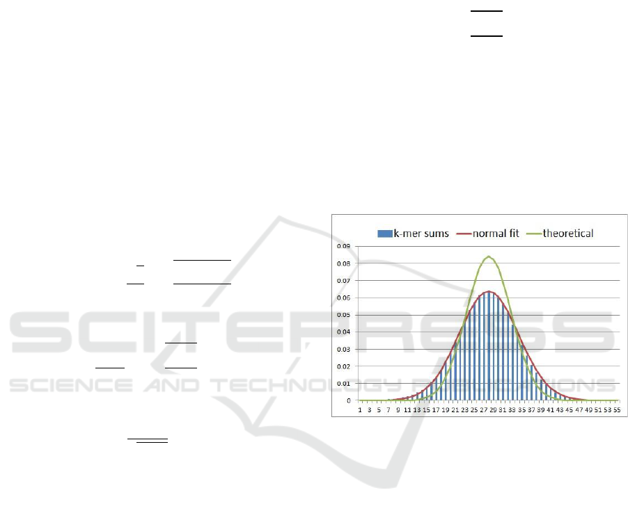
Example 2: Let k=18. Then above corollary assures
us that no more than 8.4% of data will be in the
biggest block. The corresponding variance is
and the mean value is.
Figure 1: Block size distribution for soybean data, k=18.
To see how closely these equations represent the
actual DNA data, we tested several dataset from
public domain repositories. As an example, Figure 1
illustrates the distribution of block sizes for the
Soybean data for k=18, compared with the
theoretical distribution predicted by the above
theorem. A normal fit matched the observed values
almost perfectly. Parameters for the normal fit was
and
. This yielded a peak value of
6.4%, which is close to, but less than the theoretical
upper bound of 8.4% as claimed.
For every dataset that we tested, the bell shape
has been invariant, and the peak value was around
20-25% below the theoretical value given by (4).
Looking at Figure 1, the reader can immediately
see three problems:
a. The largest block can be as big as 6.4% of the
total data size. This means that for a large data
Robust K-Mer Partitioning for Parallel Counting
149

set, the largest blocks can be too large for the
available memory.
b. The smallest block sizes are close to zero. This
means that there is a big difference between the
sizes of the largest and the smallest blocks.
c. When k-mers are individually mapped to blocks,
the sum of block sizes will reach approximately
times the size of the input data. This is because
each input line with length contains
k-mers.
The next three subsections show how to circumvent
all of these problems.
4.2 Controlling the Upper Bound
Equation (3) says that the size of the largest block is
inversely proportional to the standard deviation.
Therefore, increasing by a factor of f should
reduce
by the same factor.
One way to achieve this is by using a different
set of weights for the symbols {A, C, G, T}. For
example, instead of {0, 1, 2, 3}, use {1, 5, 10, 16}.
For this example, the range of block numbers will be
[k, 16k] instead of [0, 3k]. Consequently, will
grow by a factor of 16/3=5.33 and
will reduce
by a factor of 5.33.
Figure 2: Block size distributions for 31-mers in human
chromosome-14 for different sets of nucleotide weights.
Data has been translated to line up their mean values to aid
in visual comparison.
Actual DNA data follows this mathematical
reasoning almost precisely. As an example, Figure 2
shows the distributions of block sizes obtained from
human chromosome-14 for different sets of
nucleotide weights. In this example, k=31. For the
weight set {1, 5, 10, 16} the peak block size reduced
from 6.3% down to 1.19%. This is small enough
even for the biggest data sets encountered in
practice. In implementation, different weight sets
can be chosen depending on the amount of required
reduction for the peak value.
4.3 Converting Normal Distribution to
Uniform
The basic idea is to merge smaller blocks with larger
blocks. Thanks to the central limit theorem, we
know which blocks will be small and which blocks
will be large. If a k-mer is going to be in a small
black, re-compute its block number so that it is
mapped to a different block. In doing so, we
basically fold the tail regions of the distribution on
top of the middle region.
Let be the k-mer sum, and be the block
number for that k-mer.
Folding rule:
This rule will be applied to a k-mer iteratively as
explained below.
Here, is a positive number representing the
distance from the mean. After folding, the new block
numbers will be in the range In
discussions below, this range will be referred to as
the “target range.” Folding rule says that, if the
initially computed k-mer sum is already in the target
range, no remapping is done (third line of the
mapping rule). In this case, the k-mer sum becomes
the block number. If the k-mer sum is outside the
target range, it is mapped back into the target range,
perhaps after a few iterations.
Selection of determines the shape of the final
distribution as well as the number of iterations
needed. If is too big, there may not be enough data
in the tail regions to level up the blocks in the target
range. If is too small, tails may be too long. In
such case, a block that originally fell outside the
target range on one side may be mapped still outside
the target range on the other side. When this
happens, the folding rule will be applied again for
the new block number, and this will be repeated
until a block number inside the target range is
reached.
Figure 3 illustrates this process schematically. In
this figure the green bell shape represents the
distribution of block sizes that would be obtained
without folding. The two red bars represent the
target range. In the scenario represented in Figure 3,
the sum initially obtained for the k-mer falls
outside the target range on the left. The first time the
folding rule is applied, the computed block number
BIOINFORMATICS 2018 - 9th International Conference on Bioinformatics Models, Methods and Algorithms
150
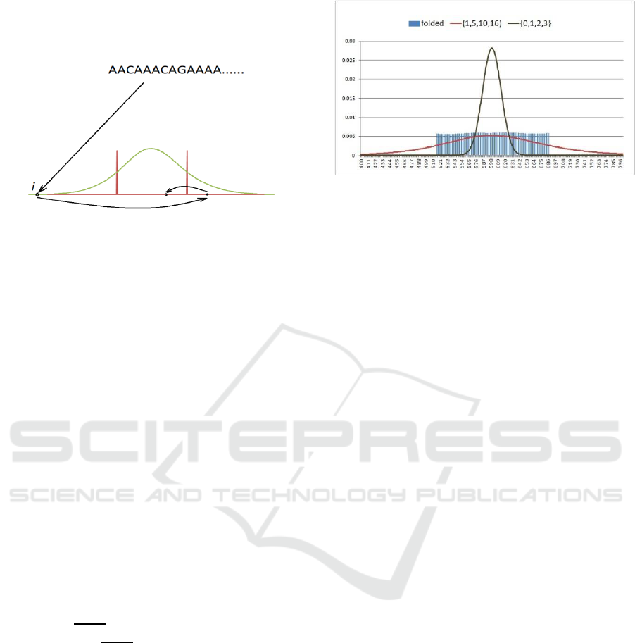
falls still outside the target range on the right. When
the folding rule is applied to this new value, the final
block number falls inside the target range.
Figure 3: Iterations of the folding rule.
Note that larger blocks outside the target range
must be close to the edge of the target range, so they
will fall near the edge inside the target range the first
time the folding rule is applied. The folding rule will
be repeated only if a block initially falls far enough
outside the target range. Since such blocks are small,
they don’t affect the shape of the final distribution.
Instead of using an iterative algorithm, it is
possible to obtain an equivalent result by using the
mod function applied to with divisor chosen as 2δ
(width of the target range). For example, the
function
maps the k-mer sum to a number in the target range
if was initially outside the target range on the left.
Similarly, the function
maps the k-mer sum to a number in the target range
if was initially outside the target range on the right.
To select consider the fact that normal
distribution reaches 50% of its peak value at
distance
from the mean. Therefore, by
selecting
we can guarantee that, after
folding, blocks at the two ends of the target range
will be about the same size as the largest block in the
middle. Bigger blocks in the target range will be
combined with smaller blocks outside the target
range. In the end, all the blocks in the target range
will have approximately equal sizes. As an example,
Figure 4 shows the result from the folding operation
for human chromosome-14 with k=75. For
comparison, distributions corresponding to weight
sets {0, 1, 2, 3} and {1, 5, 10, 16} are also shown.
The folding operation has been applied to the later
with δ computed as discussed above.
Figure 4: Block sizes obtained by the folding operation
applied to human chromosome-14.
4.4 Reducing the Total Data Size
When individual k-mers are used as the basic unit of
mapping, total data size in all the blocks blow up
from Θ(n) to Θ(kn), where is the number of lines
in the input. Without some method of compression,
this data expansion can cause a major problem when
communicating the k-mer data between processors
or when storing k-mers. The minimizers method
alleviates this problem significantly by storing line
segments instead of k-mers. If a line segment
contains k-mers sharing the same minimizer, it
must have length . We can store that line
segment instead of storing k-mers separately.
Analyses in Li et al (2013) showed that for realistic
values of and, this scheme reduces the size of k-
mer data down to Θ(n). With additional compression
techniques such as packing four nucleotides into one
byte, total data size can be reduced further.
This basic idea can be used when mapping k-mer
data into blocks. In this case, the unit of mapping
becomes the line segment instead of a k-mer. When
computing the summation formula (1), we use the p-
strings that glue together the k-mers inside line
segments. Since p-strings have fixed length, the
theoretical analysis in Section 4.1 apply without
change for the number of line segments mapped to
each block. The only modification needed is to use
as in Theorem 1.
Example 3: For the k-mers in the line segment
of Example 1, the p-string is AAT. Applying
equation (1) to this p-string, we obtain the
summation (assuming the
weight set {1,5,10,16}). Therefore, the block
number for this line segment is 18.
When applying this idea to p-strings, it is
important to ensure that is big enough for the
Central Limit theorem to take effect. To guarantee
the bell-shape, the Central Limit Theorem requires
summation of many numbers. In experiments, we
Robust K-Mer Partitioning for Parallel Counting
151
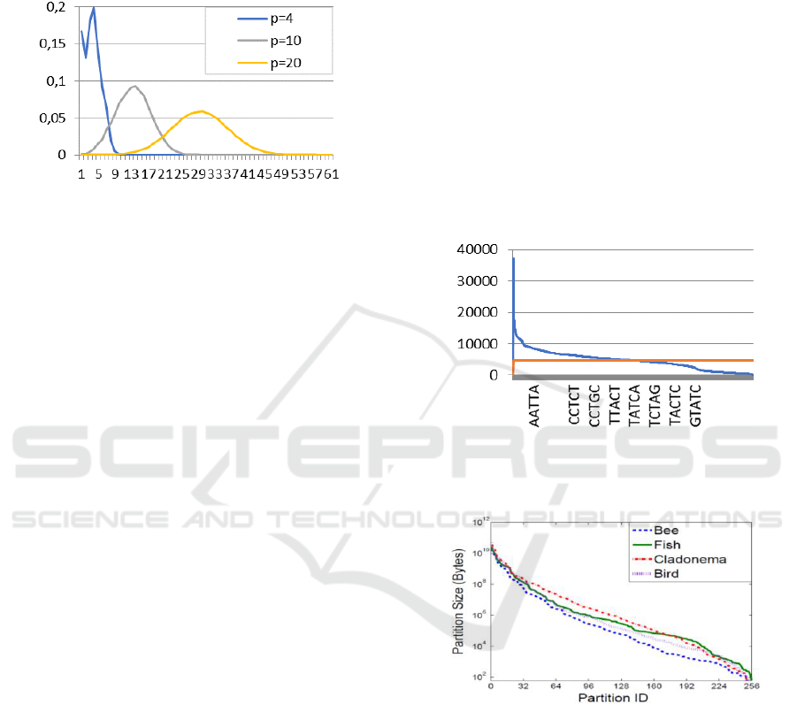
found that at around, the bell shape appears
clearly. Bigger values serve to further smooth this
shape. This is illustrated for the soybean data in
Figure 5.
Figure 5: Distribution of the number of line segments
mapped to different blocks for Soybean data with weight
set {0,1,2,3}, k=30 and different values of p.
Once the bell shape is secured, it can be
converted to a uniform distribution as described in
previous sections.
4.5 A MapReduce Algorithm for
K-Mer Counting
Various parallel counting algorithms can be
developed based on the proposed method. As an
example, a MapReduce algorithm is sketched here:
Input: Normally, input data comes in 10-15 files.
For higher parallelism divide these into hundreds of
smaller files with equal size. Each file becomes the
input for a mapper process selected at random.
Map: Each mapper process computes block
numbers and sends each line segment to its
corresponding reducer process
.
Reduce Each reducer process counts the k-mers in
the block sent to it.
5 COMPARISON WITH OTHER
METHODS
Figures 6 and 7 show the distribution of block sizes
generated by the prefix-based method, and the
minimizer-based method. A comparison with the
hash-based method is not possible, because the
authors provided no information about the hash
function used.
For the prefix-based method, we created a
computer program to generate the resulting
distributions. Figure 6 shows the case for the
soybean data. For the minimizer-based method, Li et
al., (2013) provided a histogram of block sizes for a
number of different datasets (Figure5 in their paper).
Figure 7 shows this figure. As can be seen, the
smallest block size is about 100 bytes while the
largest block size is bigger the 10 GB. The authors
suggest that increasing and then using a
“wrapping” technique will reduce the spread of
block sizes. To explain, let represent the desired
number of blocks. Wrapping here consists of
hashing the p-string that represents the name of a
block to obtain a number , and then computing
. Figure 10 in the cited paper shows the
improvement made by this method. However, the
resulting distribution still shows nearly 100-fold
difference between the sizes of the largest and the
smallest blocks.
Figure 6: Block size distribution for soybean data by the
prefix-based method: prefix length = 5, k=18. The red line
shows the median value.
Figure 7: Block size distributions by the minimizer-based
method, with p=4. (Figure reproduced with permission
from (Li et al., 2013)).
It is noted in (Erbert et al., 2017) that a variant of
the minimizer-based method generally performed
better than the original minimizer-based method
except for the FVesca dataset with k=28. For this
dataset, the method generated one very big block
about six times bigger than the next biggest block.
To see if there was some peculiar property of this
dataset which might also cause our method to fail,
we tested the proposed method on the FVesca
dataset. Figure 8 shows the result. The resulting
BIOINFORMATICS 2018 - 9th International Conference on Bioinformatics Models, Methods and Algorithms
152

distribution did contain random spikes, but the sizes
of these spikes were small.
Figure 8: Block size distribution obtained from FVesca
dataset by the proposed method with k=28.
6 CONCLUSIONS
Due to the sheer size of the input data, k-mer
counting is a memory intensive task. Equal sized
partitioning of input data is essential in order to
ensure that algorithms complete without running out
of memory. In this paper, a robust method for
partitioning input data into approximately equal
sized independent blocks has been presented.
Robustness of the proposed method follows from the
fact that distribution of k-mer sums depends on k
alone, and not the input data, as proven in Theorem
1. The mapping formulas are simple enough that
partitioning can be performed while reading the
input data from the storage medium.
Commercial software cannot be built on
algorithms that might fail occasionally. Since earlier
algorithms cannot guarantee equal block sizes, the
proposed algorithm is probably the only viable
algorithm for commercial applications.
REFERENCES
Bondarenko, B.A., 1993. Generalized Pascal triangles
and pyramids: their fractals, graphs, and applications.
Santa Clara, CA: Fibonacci Association.
Deorowicz, S., Debudaj-Grabysz, A. and Grabowski, S.,
2013. Disk-based k-mer counting on a PC. BMC
bioinformatics, 14(1), p.160.
Deorowicz, S., Kokot, M., Grabowski, S. and Debudaj-
Grabysz, A., 2015. KMC 2: fast and resource-frugal k-
mer counting. Bioinformatics, 31(10), pp.1569-1576.
Erbert, M., Rechner, S. and Müller-Hannemann, M., 2017.
Gerbil: a fast and memory-efficient k-mer counter
with GPU-support. Algorithms for Molecular
Biology, 12(1), p.9.
Li, Y., Kamousi, P., Han, F., Yang, S., Yan, X. and Suri,
S., 2013, January. Memory efficient minimum
substring partitioning. In Proceedings of the VLDB
Endowment (Vol. 6, No. 3, pp. 169-180). VLDB
Endowment.
Li, Yang, 2015. "MSPKmerCounter: a fast and memory
efficient approach for k-mer counting." arXiv preprint
arXiv:1505.06550 (2015).
Marçais, G. and Kingsford, C., 2011. A fast, lock-free
approach for efficient parallel counting of occurrences
of k-mers. Bioinformatics, 27(6), pp.764-770.
Rizk, G, D. Lavenier, R. Chikhi; 2013. DSK: k-mer
counting with very low memory usage. Bioinformatics
29 (5): 652-653. doi: 10.1093/bioinformatics/btt020.
Roberts, M., Hayes, W., Hunt, B.R., Mount, S.M. and
Yorke, J.A., 2004. Reducing storage requirements for
biological sequence comparison. Bioinformatics,
20(18), pp.3363-3369.
Smith, C. and Hoggatt, V., 1979. A study of the maximal
values in Pascals quadrinomial triangle. Fibonacci
Quarterly, 17(3), pp.264-269.
APPENDIX
Sources for the datasets mentioned in this paper:
Soybean:
http://public.genomics.org.cn/BGI/soybean_resequencing/
fastq/
Human chromosome-14:
http://gage.cbcb.umd.edu/data/
FVesca:
http://sra.dbcls.jp/search/view/SRP004241
Robust K-Mer Partitioning for Parallel Counting
153
