Building Robust Classifiers with Generative Adversarial Networks for
Detecting Cavitation in Hydraulic Turbines
Andreas Look, Oliver Kirschner and Stefan Riedelbauch
Institut f
¨
ur Str
¨
omungsmechanik und Hydraulische Str
¨
omungsmaschinen, Universit
¨
at Stuttgart, 70565 Stuttgart, Germany
Keywords:
Convolutional Neural Networks, Generative Networks, Condition Monitoring.
Abstract:
In this paper a convolutional neural network (CNN) with high ability for generalization is build. The task of the
network is to predict the occurrence of cavitation in hydraulic turbines independent from sensor position and
turbine type. The CNN is directly trained on acoustic spectrograms, obtained form acoustic emission sensors
operating in the ultrasonic range. Since gathering training data is expensive, in terms of limiting accessibility
to hydraulic turbines, generative adversarial networks (GAN) are utilized in order to create fake training data.
GANs consist basically of two parts. The first part, the generator, has the task to create fake input data, which
ideally is not distinguishable form real data. The second part, the discriminator, has the task to distinguish
between real and fake data. In this work an Auxiliary Classifier-GAN (AC-GAN) is build. The discriminator
of an AC-GAN has the additional task to predict the class label. After successful training it is possible to
obtain a robust classifier out of the discriminator. The performance of the classifier is evaluated on separate
validation data.
1 INTRODUCTION
Cavitation occurs in liquids when pressure locally
drops below vapour pressure. When such created va-
pour bubbles enter regions of higher pressure, they
will implode. This implosion can cause damage, if
the implosion happens near solid surfaces. The pro-
cess of nucleation, growth, and implosion is called
cavitation (Koivula, 2000).
In hydraulic turbines cavitation mostly occurs
when operating close to the limits of the operating
range. Often it is not clearly known whether the ma-
chinery is currently operating under cavitation condi-
tions or not. It would be advantageous to detect cavi-
tation while the turbines are running, thus the operator
can take actions in order to avoid it.
Since visual inspection of cavitation events in
hydro power plants is not possible, due to missing op-
tical accessibility, acoustic event detection offers an
alternative. Most existing cavitation detecting met-
hods rely on statistically analyzing the radiated noise,
i.e. calculating energy content in specific frequency
ranges, kurtosis, and other hand crafted features. Af-
terwards these features are examined by an expert
(Escaler et al., 2006) or fed into a classifier, e.g. SVM
(Gregg et al., 2017). These methods yield good re-
sults in laboratory environment. Representable per-
formance measurements under non laboratory condi-
tions are not available or show a dependency on the
sensor location (Schmidt et al., 2014). Therefore in
this work a robust model for detecting cavitation is
trained and evaluated. Here, robustness means, that
there is no dependency on turbine type and no or little
dependency on sensor location.
2 HARDWARE SETUP
Cavitation typically radiates noise in a broad fre-
quency range from several Hz up to the ultrasonic
range. Analyzing signals containing only information
in the ultrasonic range has the advantage of mostly
noise free signals. Noise free means, almost no influ-
ence from bearings or other mechanical parts. On the
other hand the sampling frequency has to be very high
and a lot of information has to be processed, which re-
sults in long and difficult training.
The radiated noise is recorded by acoustic emis-
sion sensors operating in the frequency range between
100 kHz and 1 MHz. Below 100 kHz the sensors be-
have like highpass filters. The upper frequency bound
is limited by the maximum sampling frequency of
2 MHz.
456
Look, A., Kirschner, O. and Riedelbauch, S.
Building Robust Classifiers with Generative Adversarial Networks for Detecting Cavitation in Hydraulic Turbines.
DOI: 10.5220/0006636304560462
In Proceedings of the 7th International Conference on Pattern Recognition Applications and Methods (ICPRAM 2018), pages 456-462
ISBN: 978-989-758-276-9
Copyright © 2018 by SCITEPRESS – Science and Technology Publications, Lda. All rights reserved

Table 1: Architecture of neural network used for conventional training. BN? indicates whether batch normalization (Ioffe and
Szegedy, 2015) was used.
Operation Kernel Strides Feature maps BN? Dropout Nonlinearity
Input N/A N/A N/A N/A N/A N/A
Convolution 3 ×3 1 ×1 8 × 0.2 ReLu
Max-Pooling 2 ×2 2 ×2 8 × × N/A
Convolution 3 ×3 1 ×1 16 × 0.2 ReLu
Max-Pooling 2 ×2 2 ×2 16 × × N/A
Convolution 3 ×3 1 ×1 32 × 0.2 ReLu
Max-Pooling 2 ×2 2 ×2 32 × × N/A
Flatten N/A N/A N/A × × N/A
Dense N/A N/A 64 × 0.2 ReLu
Dense N/A N/A 32 × × ReLu
Dense N/A N/A 1 × × Sigmoid
3 CLASSIFICATION SYSTEM
Basically it is possible to build a classifier, which
processes one-dimensional (raw signal) or two-
dimensional (spectrograms) data. Convolutional net-
works are often the best or among the best performing
neural networks in acoustic scene classification chal-
lenges (Mesaros et al., 2017; Stowell et al., 2016).
Moreover CNNs are well studied in various condi-
tion monitoring applications and are usually more of-
ten chosen (Zhao et al., 2016). Since CNNs are ori-
ginally designed for image recognition tasks, a two-
dimensional representation of the data is used.
All experiments in this work were done using Ten-
sorflow (Abadi et al., 2015).
3.1 Data Preprocessing
Before the data is used for training a classifier it has
to be preprocessed. The first step consists of applying
short-time fourier transformation (STFT) and buil-
ding spectrograms with size 512 ×384 (Frequency ×
Time). The STFT uses a Hanning window and 50 %
overlap. Thus approximately every 0,1 s one spectro-
gram is obtained. Since a wide frequency range shall
be analyzed, dynamic range compression (DCR) (Lu-
kic et al., 2016) is used in order to reduce the dyna-
mics between high and low frequencies.
f (x
i j
) = log(1 +C ·x
i j
) (1)
DCR corresponds to the elementwise application of
function 1 on every element x
i j
in a spectrogram with
C = 10
12
. C is empirically set and will not be changed
in the course of this work. For dimensional reduction
the frequency axis is wrapped by a filter bank, which
consists of 32 equally spaced and non overlapping tri-
angular windows. This method is inspired by creating
Mel-frequency cepstral coefficients, which have pro-
ven robustness in several audio recognition tasks (Sa-
hidullah and Saha, 2012). After wrapping, spectro-
grams with reduced size 32x 384 are obtained.
3.2 Conventional Training
Table 1 shows the network used for conventional trai-
ning. Conventional training in this context means, no
usage of synthetic data. The network consists of three
dense layers and three convolutional layers.
Before every layer, except the last one, dropout
(Srivastava et al., 2014) is applied in order to im-
prove the generalization capability. Additionaly after
convolution max-pooling with kernel size 2 ×2 and
stride 2 ×2 is followed. Since the task is to detect
whether cavitation occurs in the spectrogram or not,
max-pooling is useful. Basically it represents a strong
prior, stating that the occurrence of cavitation is inde-
pendent of the position in the spectrogram (Goodfel-
low et al., 2016). The kernel size of the convolutio-
nal layers is 3 ×3 with stride 1 ×1. In the first layer
8 filters, in the second 16 filters, and the third layer
32 filters are used. The network is trained using the
Adam optimizer with a learning rate of 10
−3
and ba-
tch size 16 for 40.000 weight updates, corresponding
to 70 epochs. Since the task is a classification task,
cross entropy is used as loss function.
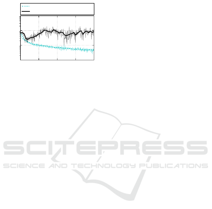
Figure 1 shows the learning curve. The whole da-
taset consists of five different hydraulic turbines. For
training purposes measurements from four different
turbines are used. Measurements from the fifth tur-
bine are part of the validation dataset. Therefore the
validation dataset consists of completely unknown
Building Robust Classifiers with Generative Adversarial Networks for Detecting Cavitation in Hydraulic Turbines
457

0 100 200 300 400
Update x100
10
−2
10
−1
10
0
10
1
Loss
Training loss
Validation loss
Figure 1: Learning curve of conventional architecture.
positions and turbine configurations. The validation
dataset consists of four different sensor positions and
has a 50/50 split between cavitation and no cavita-
tion.
According to the learning curve the training loss
decreases continuously. At the beginning of the trai-
ning the validation loss also sinks, but already shortly
after rises and then stagnates. The binary accuracy
of the validation dataset at the end of the training is
80,1 ±2,5 %. The accuracy is estimated by evalua-
ting the validation dataset 64 times with dropout and
afterwards calculating the mean and standard devia-
tion (Gal and Ghahramani, 2015). With early stop-
ping after 3500 weight updates (minimal validation
loss) a binary accuracy of 94,2 ±2,0% is obtained.
Increasing dropout rate or adding additional noise
to the inputs and hidden layers respectively often re-
present potential solutions for further increasing ge-
neralization capability, but did not succeed in this
case.
3.3 Generative Adversarial Networks
Generative adversarial networks (GAN) (Goodfellow
et al., 2014) consist of two competing neural net-
works, a generator (G) and a discriminator (D). G
takes as input random noise and outputs fake data,
which is ideally not distinguishable from real data.
The task of D is to classify the data as real or fake.
The idea of GANs can be further extended, such that
D has to identify the class label, if the sample is real,
or to classify the sample as fake. In this architecture
(SGAN) (Odena, 2016) the last layer of D is a soft-
max with N + 1 output units representing the labels
{class −1, class −2,...class −N, f ake}, where N is
the number of different classes. Using this idea it
was shown, that it is possible to train classifiers with
higher accuracy, compared to conventional training.
With fewer training data available, the better is the
advantage of using the GANs.
The problem of this method is, that the retrieved
classifier is not directly usable in real world environ-
ment, since it has learned the additional class f ake,
which does not exist in real world.
Using an auxiliary classifier GAN (AC-GAN)
(Odena et al., 2016) it is possible to circumvent this
problem. In the AC-GAN G takes an additional in-
put, which determines the class of the fake sample.
D has two different output layers. The first layer is
a softmax with N units. G predicts a class label not
only for real samples, but also for fake samples. The
second output layer is a sigmoidal, which predicts if
the sample is real or fake. The cost function therefore
consists of two parts L
S
and L
C
.
L
S
= E[log P(S = real | X
real
)]+
E[logP(S = f ake | X
f ake
)] (2)
L
C
= E[log P(C = c | X
real
)]+
E[logP(C = c | X
f ake
)] (3)
L
S
corresponds to the log-likelihood of the cor-
rect source and L
C
to the log-likelihood of the correct
class. When training D the function L
S
+ L
C
is tried
to maximize. G is trained to maximize the function
L
C
−L
S
.
The advantage of this architecture is, that a clas-
sifier, which is fit for use in real world problems, can
be directly retrieved from D. The only modification
is to remove the sigmoidal output layer, which has to
predict whether the sample is real or fake. Principally
it is also possible to retrieve a useful classifier out of
the SGAN architecture. In this case it is necessary to
replace the last layers of D, which is the softmax layer
with N +1 outputs, by a softmax layer with N outputs.
Afterwards the last few layers of the network have to
be retrained. Since this procedure seems to have no
benefits, an AC-GAN is trained in order to improve
the accuracy of the classifier.
3.3.1 Implementation
The discriminator has the same basic architecture as
already shown in table 1. One change in the architec-
ture was made by removing the last two layers. So the
network firstly outputs a 1-dimensional feature vec-
tor. This vector is then inputed into two separate neu-
ral networks with two dense layers, which predict the
class and the source of the sample. The ReLu non-
linearities have been replaced by Leaky ReLu‘s with
slope 0.1. Since the whole network, when the gene-
rator is included, has increased in depth, it is feasible
ICPRAM 2018 - 7th International Conference on Pattern Recognition Applications and Methods
458

to use Leaky ReLu‘s in order to achieve good training
results of the deep layers.
Another modification is, that the max-pooling lay-
ers have been removed. Since max-pooling would re-
sult in sparse gradients it would hinder the training
process, especially of the generator. As a compensa-
tion the stride of the convolutional layers was changed
to 2 ×2.
The architecture of the generator is shown in ta-
ble 2. G takes two inputs, the class-input z
c
and the
noise-input z
n
, and outputs one sample. z
n
is a one-
dimensional vector of size 100, drawn from a uniform
distribution with values between 0 and 1. z
c
is also a
one-dimensional vector but with size 2. In order to
connect z
n
and z
c
several possible solutions exist. In
this work the connection between these two vectors is
done via an element-wise multiplication.
Before it comes to the multiplication z
c
is em-
bedded, such that the dimension changes from 2 to
100. The embedding is done via a matrix with shape
2 ×100. The original vector z
c
indicates which of the
two vectors in the embedding matrix to choose. All
values in the matrix are also learnable parameters.
Algorithm 1 : AC-GAN Training Procedure.
Input: Number of iterations I and batch size m
for i = 1 to I do
Draw m samples from real distribution.
Update weights of D with real samples.
Draw m random samples of z
c
and z
n
.
Update weights of G.
Draw m random samples of z
c
and z
n
.
Create m synthetic samples.
Update weights of D with synthetic samples.
Draw m random samples of z
c
and z
n
.
Update weights of G.
end for
Both the generator and the discriminator have
been trained using the Adam optimizer with a decre-
ased learning rate of 10
−4
.
Algorithm 1 shows the procedure of one training
step. The training procedure consists of overall four
weight updates. Each G and D are both updated two
times. The first update of D is done using real sam-
ples, whereas the second update is done using synt-
hetic samples. G is updated both times in the same
manner.
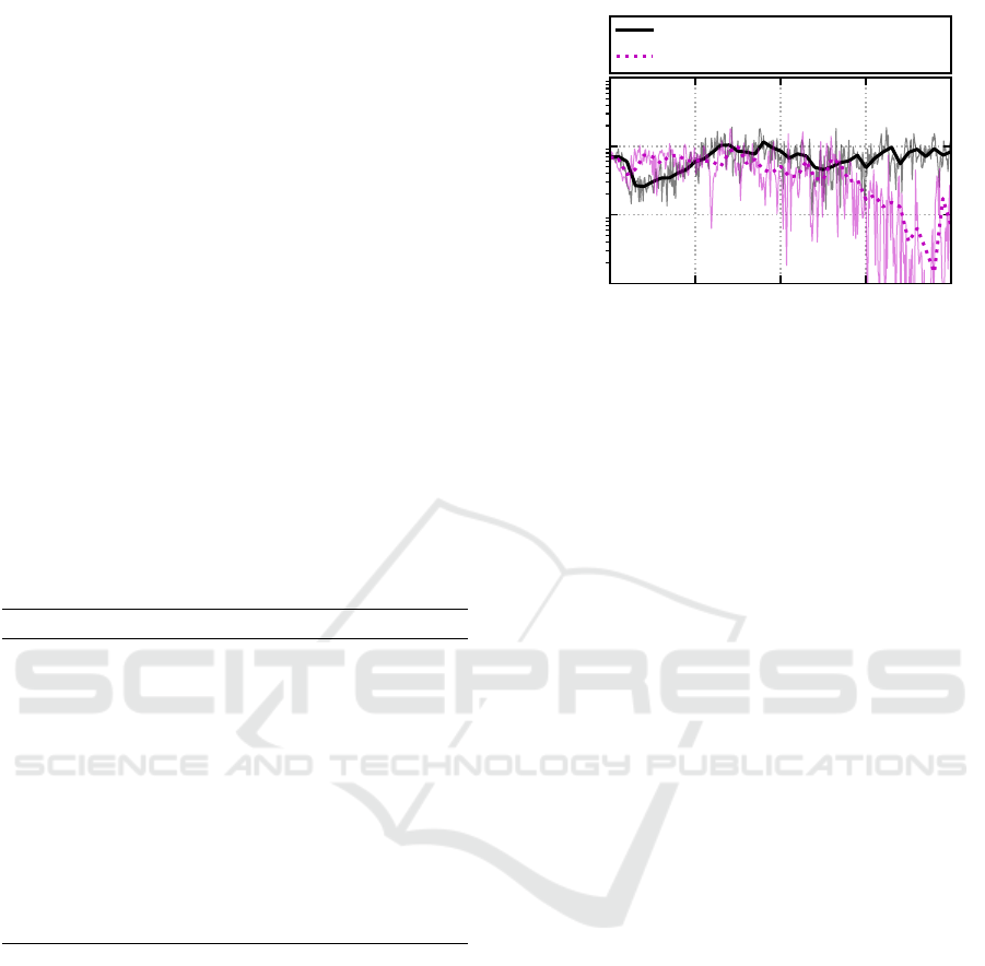
Figure 2 shows the validation loss for conventio-
nal and adversarial training. After 30.000 weight up-
dates the method using adversarial training shows cle-
arly better results. At the end of the training the ad-
versarial method has a validation loss of 0.1 (binary
accuracy of 95,1 ±1,7%) compared to a validation
0 100 200 300 400
Update x100
10
−2
10
−1
10
0
10
1
Loss
Validation loss/ Conventional
Validation loss/ AC-GAN
Figure 2: Comparison of learning curves between conventi-
onal and adversarial training.
loss of around 0.8 (binary accuracy of 80, 1 ±2,5%)
for non adversarial training. Using the adversarial
method the discriminator sees more diverse sample
and thus shows better generalization capability.
Figure 3 shows samples, which are synthesized by
the generator, in comparison to real samples. The
synthetic samples show a high similarity to the real
samples.
3.3.2 Collapsing Generators
The results shown in figure 3 have been created with
a collapsed generator. A collapsed generator means,
that the G outputs the same image, regardless of the
input. In the case of the AC-GAN architecture this
means, that G collapsed to one fixed output for each
class label. In literature feature matching (Salimans
et al., 2016) is described as an effective way to pre-
vent collapsing. When using feature matching the ob-
jective function of G is modified in a way that statis-
tics of synthetic data matches statistics of the real data
distribution. This is achieved by matching the activa-
tions of an intermediate layer of D for real and synt-
hetic samples. In this work the activations of the last
two dense layers before the final output are choosen to
match. Since the architecture used in this work con-
sists of two outputs {real?,label?} feature matching
is used for both outputs. Using this method resulted
in no significant changes in both G and D. The eva-
luation accuracy remained mostly unchanged around
95%. The collapse of G could not be prevented.
Another approach to deal with collapsing genera-
tors is to directly target diversity of synthetic samples.
Therefore the objective function of G is extended by
the additional term 4 with z
i
= [z
c
i
,z
n
i
].
E[||G(z
0
) −G(z
1
)||
2
2
] (4)
Building Robust Classifiers with Generative Adversarial Networks for Detecting Cavitation in Hydraulic Turbines
459

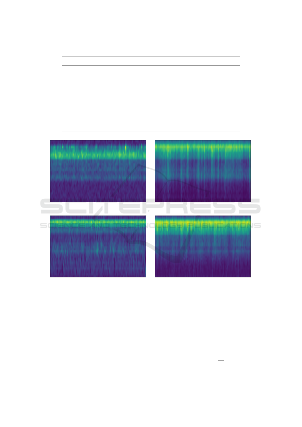
Table 2: Generator‘s architecture of the AC-GAN.
Operation Kernel Strides Feature maps BN? Dropout Nonlinearity
Class-input N/A N/A N/A N/A N/A N/A
Embedding N/A N/A N/A N/A N/A N/A
Noise-input N/A N/A N/A N/A N/A N/A
Multiplication N/A N/A N/A N/A N/A N/A
Dense N/A N/A 12288
√
× Leaky ReLu
Reshape N/A N/A N/A N/A N/A N/A
Upsampling 2 ×2 N/A N/A N/A N/A N/A
Convolution 3 ×3 1 ×1 32
√
× Leaky ReLu
Convolution 3 ×3 1 ×1 16
√
× Leaky ReLu
Convolution 3 ×3 1 ×1 16 × × Leaky ReLu
Convolution 3 ×3 1 ×1 1 × × Sigmoid
(a) no cavitation/ real (b) cavitation/ real
(c) no cavitation/ synthetic (d) cavitation/ synthetic
Figure 3: comparison between real and synthetic samples.
G is then trained to also maximize equation 4. In
essence the pixelwise variance shall be maximized
between two different inputs z
0
,z
1
under the con-
dition z
0
6= z
1
. In order to avoid cancellation bet-
ween the new additional term and the original ob-
jective function G is trained in an alternating manner.
Both terms are optimized independently from another.
Using this modified objective function the resulting
samples become very noisy and lack in dynamics (fi-
gure 4).
Since the euclidean distance depends on the abso-
lute pixel value, high values will result in high penali-
zation. Therefore G will avoid such high pixel values
and the synthetic samples lack in dynamics.
The I-divergence represents an alternative to the
euclidean distance. It is often used in the Nonnegative
Matrix Factorization problem (Finesso and Spreij,
2004). The I-divergence for two nonnegative and two-
dimensional samples X,Y is defined as:
D(X||Y ) =
∑
i, j

x
i j
log
x
i j
y
i j
−x
i j
+ y
i j

(5)
ICPRAM 2018 - 7th International Conference on Pattern Recognition Applications and Methods
460

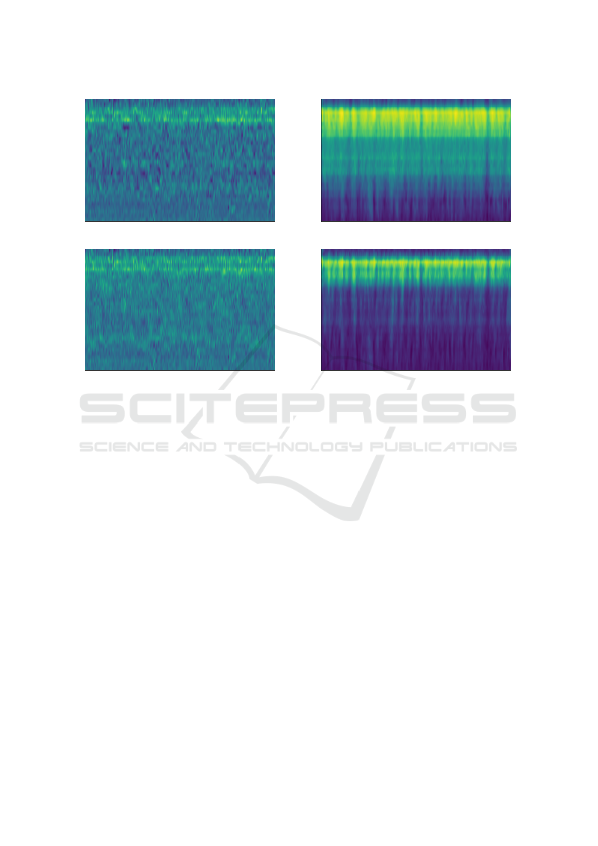
(a) cavitation/ sample 1
(b) cavitation/ sample 2
Figure 4: Synthetic samples using euclidean distance as ad-
ditional term in the objective function.
where x
i j
,y
i j
are the elements of X and Y . Like the eu-
clidean distance the I-divergence is nonnegative and
has the advantage that it is independent of the abso-
lute pixel value. In order to avoid mathematical sin-
gularities X and Y are clipped between [ε, 1], where ε
represents a small number. The new additional term
to the objective function of G is defined in equation 6.
E[D(G(z
0
)||G(z
1
))] (6)
Like before, this additional term shall be maximized
and G is trained in an alternating manner. G did not
collapse and the samples are looking realistic (figure
5). Nevertheless G did not learn the real data distribu-
tion. Several patterns resemble each other in sample 1
and 2. It seems that G learned few patterns and rand-
omly varies the intensity of these. Although not lear-
ning the real data distribution, the evaluation accuracy
could be raised to 98,1 ±1, 2 %.
Without wrapping the frequency axis experiments
mostly resulted in no collapse of G. On the downside
the evaluation accuracy dropped to 85 %. Further in-
vestigations without wrapping have to be done before
a final conclusion can be made.
(a) cavitation/ sample 1
(b) cavitation/ sample 2
Figure 5: Synthetic samples using I-divergence as additio-
nal term in the objective function.
4 SUMMARY AND OUTLOOK
In this work the usability of neural networks for de-
tecting cavitation in hydraulic machinery was shown.
Using a conventional CNN it was possible to achieve
a binary classification accuracy of 94, 2 %. Utilizing
GANs it was possible to push the classification accu-
racy to around 95,1%. Although the generator col-
lapsed, an increase in accuracy was possible. Using
the I-divergence as an additional term to the objective
function resulted in more diverse synthetic samples
and increased the accuracy to 98,1 %. In further work
the system shall be extended in such a way, that it be-
comes possible not only to detect cavitation, but also
to distinguish between different cavitation types.
ACKNOWLEDGEMENTS
The research leading to the results presented in this
paper is part of a common research project of the Uni-
versity of Stuttgart and Voith Hydro Holding GmbH.
Also we want to thank Steffen Seitz from TU Dresden
for the helpful exchange of ideas.
Building Robust Classifiers with Generative Adversarial Networks for Detecting Cavitation in Hydraulic Turbines
461

REFERENCES
Abadi, M., Agarwal, A., Barham, P., Brevdo, E., Chen, Z.,
Citro, C., Corrado, G. S., Davis, A., Dean, J., De-
vin, M., Ghemawat, S., Goodfellow, I., Harp, A., Ir-
ving, G., Isard, M., Jia, Y., Jozefowicz, R., Kaiser,
L., Kudlur, M., Levenberg, J., Man
´
e, D., Monga, R.,
Moore, S., Murray, D., Olah, C., Schuster, M., Shlens,
J., Steiner, B., Sutskever, I., Talwar, K., Tucker, P.,
Vanhoucke, V., Vasudevan, V., Vi
´
egas, F., Vinyals, O.,
Warden, P., Wattenberg, M., Wicke, M., Yu, Y., and
Zheng, X. (2015). Tensorflow: Large-scale machine
learning on heterogeneous systems.
Escaler, X., Egusquiza, E., Farhat, M., Avellan, F., and
Coussirat, M. (2006). Detection of cavitation in hy-
draulic turbines. Mechanical systems and signal pro-
cessing, 20(4):983–1007.
Finesso, L. and Spreij, P. (2004). Nonnegative matrix fac-
torization and i-divergence alternating minimization.
Gal, Y. and Ghahramani, Z. (2015). Dropout as a baye-
sian approximation: Representing model uncertainty
in deep learning.
Goodfellow, I., Bengio, Y., and Courville, A. (2016). Deep
Learning. MIT Press.
Goodfellow, I., Pouget-Abadie, J., Mirza, M., Xu, B.,
Warde-Farley, D., Ozair, S., Courville, A., and Ben-
gio, Y. (2014). Generative adversarial networks.
Gregg, S., Steele, J., and Van Bossuyt, D. (2017). Machine
learning: A tool for predicting cavitation erosion rates
on turbine runners. Hydro Review, 36(3):28–36.
Ioffe, S. and Szegedy, S. (2015). Batch normalization:
Accelerating deep network training by reducing inter-
nal covariate shift.
Koivula, T. (2000). On cavitation in fluid power. In Procee-
dings of 1st FPNI-PhD Symposium.
Lukic, Y., Vogt, C., Durr, O., and Stadelmann, T. (2016).
Speaker identification and clustering using convoluti-
onal neural networks. In IEEE International Confe-
rence on Acoustic, Speech and Signal Processing.
Mesaros, A., Heittola, T., Diment, A., Elizalde, B., Shah,
A., Vincent, E., Raj, B., and Virtanen, T. (2017).
DCASE 2017 challenge setup: Tasks, datasets and ba-
seline system. In Proceedings of the Detection and
Classification of Acoustic Scenes and Events 2017
Workshop (DCASE2017).
Odena, A. (2016). Semi-supervised learning with genera-
tive adversarial networks.
Odena, A., Olah, C., and Shlens, J. (2016). Conditional
image synthesis with auxiliary classifier gans.
Sahidullah, M. and Saha, G. (2012). Design, analysis
and experimental evaluation of block based transfor-
mation in mfcc computation for speaker recognition.
Speech Communication, 54(4):543 – 565.
Salimans, T., Goodfellow, I., Zaremba, W., Cheung, V.,
Radford, A., and Chen, X. (2016). Improved techni-
ques for training gans.
Schmidt, H., Kirschner, O., and Riedelbauch, S. (2014). In-
fluence of the vibro-acoustic sensor position on cavita-
tion. In Proceedings of 27th Symposiom on Hydraulic
Machinery and Systems.
Srivastava, N., Hinton, G., Krizhevsky, A., Sutskever, I.,
and Salakhutdinov, R. (2014). Dropout: A simple way
to prevent neural networks from overfitting. Journal
of Machine Learning Research, 15:1929–1958.
Stowell, D., Wood, M., Stylianou, Y., and Glotin, H. (2016).
Bird detection in audio: a survey and a challenge.
Zhao, R., Yan, R., Chen, Z., Mao, K., Wang, P., and Gao, R.
(2016). Deep learning and its applications to machine
health monitoring: A survey.
ICPRAM 2018 - 7th International Conference on Pattern Recognition Applications and Methods
462