Earth Mover’s Distances for Rooted Labaled Unordered Trees based on

Tai Mapping Hierarchy

Taiga Kawaguchi and Kouichi Hirata

Kyushu Institute of Technology, Kawazu 680-4, Iizuka 820-8502, Japan

Keywords:

Earth Mover’S Distance, Rooted Labeled Unordered Tree, Tai Mapping Hierarchy, Tree Edit Distance.

Abstract:

In this paper, we introduce earth mover’s distances (EMDs, for short) for rooted labeled trees based on Tai

mapping hierarchy. First, by focusing on the restricted mappings in the Tai mapping hierarchy providing the

tractable variations of the tree edit distance, we formulate the EMDs whose signatures are all of the pairs of a

complete subtree and its frequency and whose ground distances are the tractable variations. Then, we compare

the EMDs with their ground distances, which are tractable variations.

1 INTRODUCTION

Comparing tree-structured data such as HTML and

XML data for web mining or DNA and g lycan d ata

for bioinformatics is one of the important task s for

data mining. The most famous distance measure bet-

ween rooted labeled unordered trees (trees, for short)

is the edit distance (Tai, 1979). The edit distance is

formu late d as the minimum c ost of edit operations,

consisting of a substitution, a deletion and an inser-

tion, applied to transform from a tree to another tree.

Whereas the edit distance is a metric, the problem of

computing the edit distan ce is MAX SNP-hard even if

trees are binary (Hirata et al., 2011; Zhang a nd Jiang,

1994).

As constant-factor low er bounding distances of

the edit distance, several histogram distances based

on local information (Aratsu et al., 2009; Kailing

et al., 2004; Li et al., 2013) have introduced. Whe-

reas w e can co mpute them more efﬁciently than the

edit distance, none of them is a metric.

On the other hand, an earth mover’s distance

(EMD, for short) has originally d eveloped to com-

pare with two images in image retrieval and pattern

recogn ition (Rubner et al., 2007) and is formulated

as the solution of the transportation problem between

the distributions of fe a tures in signatures in two ima-

ges. It is known that the EMD is a metric if so is the

ground distance between single features.

Gollapudi and Panigrahy (Gollapudi and Pani-

grahy, 2008) have extended the EMD to th at between

two leaf-labeled trees with the same height, whe re a

tree is leaf-labe led if all of the labels are assigned to

just leaves. However, it is difﬁcult for the EM D to

extend to be applica ble to standard two trees, that is,

labels are assigned to all the nodes and having possi-

ble different height as follows. In the EMD, ﬁrst, by

comparing each pair of leaves (that is, the nodes with

height 1), we set the value 1 if both leaves have the

same label and 0 otherwise. Then, by using the infor-

mation between the pair of nodes in the height k − 1,

we solve the transportation problem of the pair of no-

des in the height k. Hence, in order to apply such a

recursion to tre es, the trees are ne c essary to have the

same height and have no internal nodes with labels.

Kawaguchi and Hirata (Kawaguchi and Hirata,

2017) have introdu ced another EMD based on com-

plete subtrees. The EMD is formulated by the his-

tograms consisting of either c omplete subtrees, co-

complete subtree or both and their frequencies as sig-

natures a nd the L

-distance between the h isto grams as

ground distances, so we can apply the EMD to rooted

labeled trees. Also the E MD is a metric and tracta-

ble. On the other hand, there exist trees that the EMD

cannot reﬂect intuitive similarity.

Since the edit distance betwe e n trees is corre-

sponding to a Tai mapping ( Tai, 1979 ), many vari-

ations of th e edit distan c e have developed as more

structurally sensitive distances obtained by restricting

the Tai mapping, that is, a top-down distance (Cha-

wathe, 1999; Selkow, 1977 ), an LCA- and root-

preserving distance (Yoshino and Hirata, 2017), an

LCA-preserving distance (Zhang et al., 1996), an

accordant distance (Kuboyama, 2007), an isolated-

subtree (or a constrained) distance (Zhang, 1995;

Zhang, 1996) and an alignment distance (Jiang et al.,

Kawaguchi, T. and Hirata, K.

Earth Mover’s Distances for Rooted Labaled Unordered Trees based on Tai Mapping Hierarchy.

DOI: 10.5220/0006633701590168

In Proceedings of the 7th International Conference on Pattern Recognition Applications and Methods (ICPRAM 2018), pages 159-168

ISBN: 978-989-758-276-9

159

1995). Almost variations are metrics except an align-

ment distance (Jiang et al., 1995). Also, whereas the

problem of computing the edit distance or the align-

ment distance between trees is MAX SNP-hard (Hi-

rata et al., 2011; Jiang et al., 1995; Zhang and Jiang,

1994), the problem of computing the other variations

is tractable.

The reason why these variations are tractable is

that the maximum weight bipartite matching pro-

blem can be applied to computing the variations after

decomp osing trees from the root (Yamamoto et al.,

2014). In contrast, it cannot b e applied to computing

the edit distance and the alignm e nt distance, because

computing them is necessary to compare the decom-

posed trees and the remained tre es after decomposin g

trees from the root.

Since we can regard the minimum weig hted b i-

partite pro blem as a special case of the transportation

problem in EMDs, in this paper, we formulate new

EMDs based on the Tai mapping hierarchy whose sig-

natures are pairs of a complete subtree and the ratio

of frequencies oc c urring in a whole tree and whose

ground distances are the tractable variations of the

edit distance . Then, we show that the EMDs are al-

ways metrics and tractable. Finally, we give experi-

mental results to evaluate the EMDs to compare them

with their ground distanc es and investigate the pro-

perties of the E MDs.

2 PRELIMINARIES

A tree T is a connected graph (V,E) without cycles,

where V is the set of vertices and E is the set of edges.

We denote V an d E by V (T ) and E(T ). The size of

T is |V | and denoted by |T |. We sometime denote

v ∈ V (T ) by v ∈ T . We denote an empty tree (

0) by

0. A rooted tree is a tree with one node r chosen as its

root. We d e note the root of a rooted tree T by r(T ).

For each node v in a rooted tree with the root r,

let UP

(v) be the unique path from v to r. The pare nt

of v(6= r), which w e denote by p ar(v), is its adjacent

node on UP

(v) and the a ncestors of v(6= r) are the

nodes on UP

(v) − {v}. We denote the set of all an-

cestors of v by anc(v). We say th at u is a child of v if

v is the parent of u and u is a descendant of v if v is

an ancestor of u. We use the ancestor orders < and ≤,

that is, u < v if v is an ancestor of u and u ≤ v if u < v

or u = v. We say that w is the least common ancestor

of u and v, denoted by u ⊔ v, if u ≤ w, v ≤ w a nd there

exists no w

′

such that w

′

≤ w, u ≤ w

′

and v ≤ w

′

. is

the numb er of children of v. The degree of a rooted

tree T , denoted by d(T ), is the maximum number of

d(v) for every v ∈ T .

For n odes u,v ∈ T , u is to the left of v if pre(u) ≤

pre(v) for the preorder number pre and post(u) ≤

post(v) for the postor der number post. We say that

a rooted tree is ordered if a lef t-to-right order among

siblings is given; unordere d oth e rwise. We say that a

rooted tree is labeled if each node is assigned a sym-

bol from a ﬁxed ﬁnite alphabet Σ. For a node v, we

denote the labe l o f v by l(v), and sometimes identif y

v with l(v). In this paper, we call a rooted labeled

unordered tree a tree simply.

Let T be a tree (V , E) and v a node in T . A com-

plete subtree of T at v, de noted by T [v], is a tree

′

= (V

′

) such that r(T

′

) = v, V

′

= {u ∈ V | u ≤ v}

and E

′

= {(u,w) ∈ E | u,w ∈ V

′

}. We denote the

(multi)set {T [v] | v ∈ T } of all the com plete subtrees

in T by cs(T ). For a complete subtree S in T , we

denote the frequency of the occurrences of S in T by

f (S,T ).

Next, we introduce an edit distance an d a Tai map-

ping.

Deﬁnition 1 (Edit operations (Tai, 1979)). The edit

operations of a tree T are deﬁned as follows. (Fi-

gure 1).

1. Substitution: Change the label of the node v in T .

2. Deletion: Delete a node v in T with parent v

′

, ma-

king the children of v become the childr en of v

′

The children are inserted in the place of v as a sub-

set of the children of v

′

. In particular, if v is the

root in T , then th e result apply ing the deletion is a

forest consisting of the children of the root.

3. Insertion: The complement of deletion. Insert a

node v as a child of v

′

in T making v the parent o f

a subset of the children of v

′

Substitution (v 7→ w)

7→

Deletion (v 7→ ε)

′

7→

′

Insertion (ε 7→ v)

′

7→

′

Figure 1: Edit operations for trees.

Let ε 6∈ Σ denote a special blank symbol and d eﬁne

= Σ ∪ {ε}. Then, we represent each edit operation

ICPRAM 2018 - 7th International Conference on Pattern Recognition Applications and Methods

160

by (l

7→ l

), where (l

) ∈ (Σ

×Σ

−{(ε,ε)}). The

operation is a substitution if l

6= ε and l

6= ε, a dele-

tion if l

= ε, and an insertion if l

= ε. For n odes u

and v, we also denote (l(u) 7→ l(v)) by (u 7→ v). We

deﬁne a c ost function γ : (Σ

×Σ

−{(ε,ε)}) 7→ R

pairs of labels. We often c onstrain a cost function γ to

be a metric, that is, γ(l

) ≥ 0, γ(l

) = 0 iff l

= l

γ(l

) = γ(l

) an d γ(l

) ≤ γ(l

)+γ(l

). In

particular, we call the cost functio n that γ(l

) = 1

if l

6= l

a unit cost function.

Deﬁnition 2 (Edit distance (Tai, 1979)). For a cost

function γ, the c ost of an edit operation e = l

7→ l

is given by γ(e) = γ(l

). The cost of a sequence

E = e

,... ,e

of edit operations is given by γ(E) =

∑

i=1

γ(e

). Then, an edit distance τ

TA I

) bet-

ween trees T

and T

is deﬁned as follows:

TA I

)

= min







γ(E)



E is a sequence

of edit operations

transforming T

to T







Deﬁnition 3 (Tai mapping (Tai, 1979)). Let T

and

be tree s. We say that a triple (M, T

) is an unor-

dered Tai mapping (a mapping, for short) from T

if M ⊆ V (T

) × V (T

) and every pair (u

) and

) in M satisﬁes that (1) u

= u

iff v

= v

(one-

to-one condition) a nd (2) u

≤ u

iff v

≤ v

(ancestor

condition). We will use M instead of (M,T

) when

there is no confusion denote it by M ∈ M

TA I

Let M be a mapping from T

to T

. Let I

and J

be the sets of nodes in T

and T

but not in M, that is,

= {u ∈ T

| (u,v) 6∈ M} and J

= {v ∈ T

| (u,v) 6∈

M}. Then, the cost γ(M) of M is given as follows.

γ(M) =

∑

(u,v)∈M

γ(u,v) +

∑

u∈I

γ(u,ε) +

∑

v∈J

γ(ε,v).

Theorem 1. The following statement holds (Tai,

1979).

TA I

) = min{γ(M) | M ∈ M

TA I

)}.

Unfortu nately, the following theorem holds for

computing τ

TA I

between unordered trees.

Theorem 2. For uno rdered trees T

and T

, the

problem of computing τ

TA I

) is MAX SNP-

hard (Zhang and Jiang, 1994). This statement also

holds even if both T

and T

are binary (Hirata et al.,

2011).

Finally, we introduce the variations of a Tai map-

ping and an edit distance.

Deﬁnition 4 (Variations of Tai mapping). Let T

and

be trees and M ∈ M

TA I

). We denote M \

{(r(T

),r(T

))} by M

−

1. We say that M is an isolated-subtree map-

ping (Zhang, 1995; Zhang, 1996), denoted by

M ∈ M

ILST

), if M satisﬁes the following

condition.

∀(u

)(u

) ∈ M

< u

⊔ u

⇐⇒ v

< v

⊔ v

2. We say that M is a n accordant mapping (Ku-

boyama, 2007), denoted by M ∈ M

ACC

), if

M satisﬁes the following con dition.

∀(u

)(u

) ∈ M

⊔ u

= u

⊔ u

⇐⇒ v

⊔ v

= v

⊔ v

3. We say that M is an LCA-preserving map-

ping (Zhang et al., 1996), denoted by M ∈

LCA

), if M satisﬁes the following condi-

tion.

∀(u

)(u

) ∈ M ((u

⊔ u

⊔ v

) ∈ M) .

4. We say that M is an LCA- and root-preserving

mapping (Yoshino a nd Hirata, 2017) , denoted by

M ∈ M

LCART

), if M ∈ M

LCA

) and

(r(T

),r(T

)) ∈ M.

5. We say that M is a Top-down mapping (Ch a-

wathe, 1999; Selkow, 1977), denoted by M ∈

TOP

), if M satisﬁes the following condi-

tion.

∀(u,v) ∈ M

−

((par(u),par (v)) ∈ M).

The above variation of Tai mapping provides the

following hierarchy (Kuboyama , 2007; Yoshino and

Hirata, 2017).

TOP

) ⊆ M

LCART

) ⊆ M

LCA

)

⊆ M

ACC

) ⊆ M

ILST

) ⊆ M

TA I

Deﬁnition 5 (Variations of e dit distance). For every

A ∈ {ILST, ACC, LCA, LCART, TOP}, we deﬁne the

distance τ

) as follows.

) = min {γ(M ) | M ∈ M

)}.

Here we call τ

ILST

an isolated-subtree dis-

tance (Zhang, 1995; Zhang, 1996), τ

ACC

an accordant

distance (Kuboyam a , 2007 ), τ

LCA

an LCA-preserving

distance (Zha ng et al., 1996), τ

LCART

an LCA- and

root-preserving distance (Yoshino and Hirata, 2017),

and τ

TOP

a top-down distance (Chawathe, 1999; Sel-

kow, 1977). By the Tai mapping hierarchy, the fol-

lowing inequality for the variation of edit distanc e

holds.

TA I

) ≤ τ

ILST

) ≤ τ

ACC

) ≤

LCA

) ≤ τ

LCART

) ≤ τ

TOP

Furthermore, f or all the above variations, the follo -

wing theorem holds.

Earth Mover’s Distances for Rooted Labaled Unordered Trees based on Tai Mapping Hierarchy

161

Theorem 3 (cf., (Yamamoto et al., 2014; Yoshino and

Hirata, 2017; Zhang et al., 1996)). For every A ∈

{ILST, ACC, LCA, LCART, TOP}, we can compute

) in O(n

d) time, where n = max (|T

|,|T

and d = min{d(T

),d(T

)}.

3 EARTH MOVER ’S DISTANCE

FOR TREES

In this section , we ﬁrst introduce an earth mover’s dis-

tance (Rubner et a l., 20 07) and then extend to that for

trees based on Tai mapp ing hierarc hy.

We call the set of pairs of a fe a ture p

and its

weight w

a signature and denote it by P = {(p

)}.

For a feature p

such that (p

) ∈ P, we denote

∈ P simp ly. An earth mover’s distance (EMD, for

short) between two signature s is given as the mini-

mum cost of the transportation problem fr om a signa-

ture to another signature.

Let P = {(p

)} and Q = {(q

)} be signatu-

res. We call a distance between p

and q

a grou nd

distance and denote it by gd(p

). Also w e denote

the ﬂow from p

to q

by f

i j

. Whe n the cost of the ﬂow

from p

to q

is given by gd(p

) f

i j

, the overall cost

of the ﬂows from P to Q is deﬁned as follows.

∑

∈P

∑

∈Q

gd(p

) f

i j

Then, ﬁnd the minimum cost ﬂow f

∗

i j

subject to the

following constraints:

1. f

i j

≥ 0,

∑

∈P

i j

≤ u

∑

∈Q

i j

≤ v

∑

∈P

∑

∈Q

i j

= min



∑

∈P

∑

∈Q



The constraint (1) allows moving “ supplies” from P

to Q and not vice versa. The co nstraints (2) and (3)

limit the amount of supp lies within the weight. The

constraint (4) forces to move the maximum amount

of supplies possible.

Let f

∗

i j

be the optimum ﬂow of the transportation

problem. Then, we deﬁne the EMD between two sig-

natures P and Q as follows.

EMD

(P,Q) =

∑

∈P

∑

∈Q

gd(p

) f

∗

i j

∑

∈P

∑

∈Q

∗

i j

∑

∈P

∑

∈Q

gd(p

) f

∗

i j

min



∑

∈P

∑

∈Q



Note that the EMD allows for partial matches

when the total weight of a signature is different from

that of another signature, which is impor ta nt for

image retrieval applications (Rubner et al., 2007). We

can realize the partial match to transpo rt from a signa-

ture whose total we ight is smaller than a part of anot-

her signature. Also the following theor em holds for

the EMD.

Theorem 4. Suppose that two signatures have the

same total weight. If a ground distance is a me-

tric, then so is the EMD. F urthermore, we can

compute the EMD in O(n

log n) time, where n =

max{|P|,|Q|} (Rubner et al., 2007).

Next, we formulate the E MD for trees based on

Tai ma pping hie rarchy.

It is necessary for the EMD to introduce a signa-

ture and a groun d distance between features. In order

to fo rmulate the EMD for trees, we transform from a

tree to a signature. In this p aper, we adopt the follo-

wing signature s(T ) for a tree T .

s(T ) =



(S,w)



S ∈ cs(T ), w =

f (S,T )

|T |



The features of s(T ) are complete subtrees of T and

the weight of s(T ) is the ratio of the occurrences of

complete subtrees. Hence, the total weight of s is 1.

Since this signature contains T itself, we can trans-

form T to s(T ) uniquely. On the other hand, as a

ground distance between trees, we adopt 5 tractable

variations of the edit distance, that is, τ

TOP

, τ

LCART

LCA

, τ

ACC

and τ

ILST

Hence, by combinin g signatures and ground dis-

tances, we formalize the following 5 kinds of an

EMD for trees. In the following, we assume that

A ∈ {ILST, ACC, LCA, LCART, TOP}.

Deﬁnition 6 (EMD for trees) . We deﬁne an EMD

for trees as EMD

(s(T

),s(T

)) betwee n signatures

s(T

) and s(T

) for a ground distance τ

and denote it

by EMD

Corollary 1. EMD

) is a metr ic .

Proof. It is straightforward since a ground distance

is a metric and the total weight of signatures is 1

and by Theorem 4.

Theorem 5. We can compute EMD

) in

O(n

logn) time, where n = max{|T

|,|T

|}.

Proof. By u sing s(T

), s(T

) and {τ

[u],T

[v]) |

(u,v) ∈ T

× T

}, we can design the following algo-

rithm to compute EMD

1. Co nstruct s(T

) and s(T

) from T

and T

2. Co mpute G = {τ

[u],T

[v]) | (u, v) ∈ T

× T

3. Co mpute EMD

) from G.

ICPRAM 2018 - 7th International Conference on Pattern Recognition Applications and Methods

162

It is obvious th at the running time of Step 1 is

O(n). For Step 2, since the algorithm of computing

) can store the value of τ

[u],T

[v]) for

every (u,v) ∈ T

×T

and by Theorem 3, w e can com-

pute G in O(n

d) time, where d = min {d(T

),d(T

)}.

Since |s(T

)| = |s(T

)| = O(n) and by Theo rem 4,

the running time of Step 3 is O(n

logn). Hence,

we can compute EMD

) in O(n) + O(n

d) +

O(n

logn) = O(n

logn) time.

4 EXPERIMENTAL RESU LTS

In this section, we give experimental results to evalu-

ate EMD

to compar e EMD

with τ

and investigates

the properties of EMD

. He re, we assume that a cost

function is a unit cost function.

In this section, we use two kinds of data; One is N-

glycan data provided from KEGG

as real data. Anot-

her is 6 data of randomly generated trees by using the

algorithm PTC (Luke and Panait, 2001). We call them

(1 ≤ i ≤ 6), where the number of nodes in R

50 × i. Furthermore, we use the computer environ-

ment that CPU is Intel Xeon E51650 v3 (3.50GHz),

RAM is 1GB and OS is Ubuntsu Linux 14. 04 (64bit).

Table 1 illustrates the details of data, that is, the

number of data (#), the average number of nodes (n),

the average degre e (d) a nd the average heig ht (h).

Table 1: The details of data.

data # n d h

N-glycan 2142 11.07 2.07 6.20

100 50.00 2.00 8.75

100 100.00 2.00 10.69

100 150.00 2.00 12.12

100 200.00 2.00 12.75

100 250.00 2.00 13.81

100 300.00 2.00 14.24

4.1 Running Time

First, we compare the running time to co mpute EMD

and τ

for N-glycan data and randomly generated

trees in Table 1. Table 2 illustrates the running time

to compute such distances.

Tables 1 and 2 show that the running time of both

EMD

and τ

is increasing when the numbe r of nodes

is increasing and the ratio of increasing for EMD

larger than that for τ

Kyoto Encyclopedia of Genes and Genomes.

http://www.kegg.jp/

Table 2: The running time to compute the distances (sec.).

distance N-glycan R

ILST

1580.95 69.72 289.48

ACC

1386.33 60.18 285.78

LCA

1129.97 49.13 201.78

LCART

1109.80 49.64 203.96

TOP

485.42 20.71 83.56

EMD

ILST

1592.32 77.00 351.81

EMD

ACC

1399.14 66.23 307.31

EMD

LCA

1133.82 55.17 261.24

EMD

LCART

1128.05 55.08 261.36

EMD

TOP

509.49 26.45 138.04

distance R

ILST

665.12 118 6.53 187 4.17 272 2.80

ACC

578.79 101 3.98 159 7.39 230 8.71

LCA

461.58 824.09 1298.07 1873.32

LCART

467.38 834.47 1313.06 1891.92

TOP

189.58 336.86 527 .42 760. 66

EMD

ILST

894.53 180 2.92 307 3.49 483 2.80

EMD

ACC

790.38 158 3.50 276 3.23 437 6.64

EMD

LCA

687.20 140 1.26 247 4.14 396 5.60

EMD

LCART

687.29 141 4.33 247 4.22 396 1.98

EMD

TOP

397.84 875.98 1637.42 2759.20

Table 3 illustrates the ratio (EMD

/τ

) of the run-

ning time of computing the EMDs (EMD

) for that of

computing the ground distances (τ

) in Table 2. Here,

we call it the ratio of EMD

for τ

simply.

Table 3: The ratio (EMD

/τ

) of the running time of com-

puting the EMDs (EMD

) for that of computing the ground

distances (τ

) in Table 2.

A N-glycan R

ILST 1.01 1.10 1.22 1.34 1.52 1.64 1.77

ACC 1.01 1.10 1.08 1.37 1.56 1.73 1.90

LCA 1.00 1.12 1.29 1.49 1.70 1.91 2.12

LCART 1.02 1.11 1.28 1.47 1.69 1.88 2.09

TOP 1.05 1.28 1.65 2.10 2.60 3.10 3.63

Table 3 shows that, w hereas the ratio of EMD

for

is between 1.00 and 1.05 for N-glycan data, the ra-

tio of EMD

TOP

for τ

TOP

is over 3 for the data R

. On

the other hand, smaller distance in the inequality for

the variations (τ

ILST

≤ τ

ACC

≤ τ

LCA

≤ τ

LCART

≤ τ

TOP

)

tends to give smaller ra tio of EMD

for τ

except

LCA and LCART; The ratio of EMD

LCA

for τ

LCA

greater than the ratio of EMD

LCART

for τ

LCART

Furthermore, whereas the ratio of EMD

for τ

O(nlog n/d) in theoretical by Theorems 3 and 5, the

ratio is at most 4 in experimental. Then, the problems

Earth Mover’s Distances for Rooted Labaled Unordered Trees based on Tai Mapping Hierarchy

163

of computing EMDs are e fﬁcient for trees with at least

300 nodes and small d egre e.

4.2 Comparing EMDs with Ground

Distances

Next, we investigate the relationship between the

EMD EMD

and its ground distance τ

for N-glycan

data.

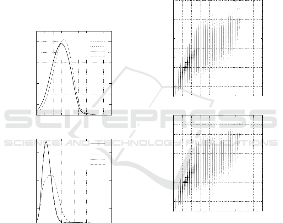
Figure 2 illustrates the distributions of E MDs (up-

per) and ground distances (lower). Here, the x-axis is

the value of the distance and the y-axis is the percen-

tage of pairs with the distance pointed by the x-axis.

0 1 2 3 4 5 6 7 8 9

percentage(%)

distance

EMD_Ilst

EMD_Acc

EMD_Lca

EMD_LcaRt

EMD_Top

0 10 20 30 40 50 60

percentage(%)

distance

Ilst

Acc

Lca

LcaRt

Top

Figure 2: The distributions of EMDs (upper) and ground

distances (lower) for N-glycan data.

Figure 2 shows that both EMDs and gr ound dis-

tances are near to normal distribution. Also the distri-

butions of EMD

TOP

and τ

TOP

are right to other EMD

and τ

(A ∈ {ILST, ACC, LCA, LCART}), respecti-

vely. Whereas the peak of the distribution of EMD

TOP

is larger than that of other distributions of EMD

, the

peak of the distribution of τ

TOP

is smaller than that of

other distributions of τ

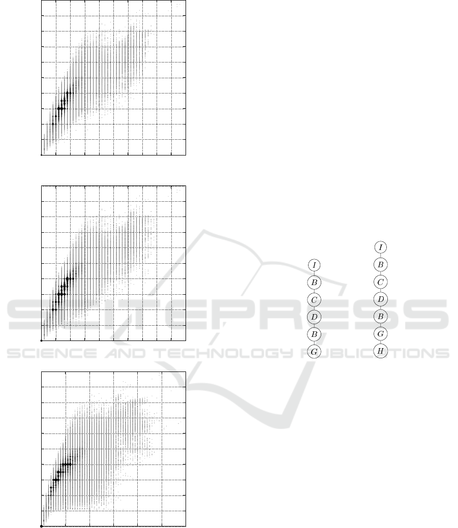
Figures 3 and 4 illustrate the scatter charts bet-

ween the number of pairs of trees with τ

pointed

at the x-axis and that with EMD

pointed at the y-

axis for N-g lycan data whose number of total pairs is

2,293,011. Here, the diameter a nd th e colo r represent

the number of pairs of trees such that longer diameter

and deeper color are larger number. Also, Figures 3

and 4 represent the cases that A ∈ {ILST, ACC} and

A ∈ {LCA, LCART, TOP}, respectively.

0 5 10 15 20 25 30 35 40 45 50

ILST

0 5 10 15 20 25 30 35 40 45 50

ACC

Figure 3: The scatter charts between the number of pairs

of trees with τ

pointed at the x-axis and that with EMD

pointed at the y-axis for A ∈ {ILST, ACC}.

Figures 3 and 4 show that EMD

is relative to

and almost values of τ

are larger tha n those of

EMD

. Also the plots of TOP vary more widely than

others.

4.3 Typical Cases

In the following, we point out the typical cases of

trees with different values between of τ

and EMD

ICPRAM 2018 - 7th International Conference on Pattern Recognition Applications and Methods

164

0 5 10 15 20 25 30 35 40 45 50

LCA

0 5 10 15 20 25 30 35 40 45 50

LCART

0 10 20 30 40 50 60

TOP

Figure 4: The scatter charts between the number of pairs

of trees with τ

pointed at the x-axis and that with EMD

pointed at t he y-axis for A ∈ {LCA, LCART, TOP}.

Here, let u

be a node in T

such that pre(u

) = i and

a node in T

such that pre(v

) = i.

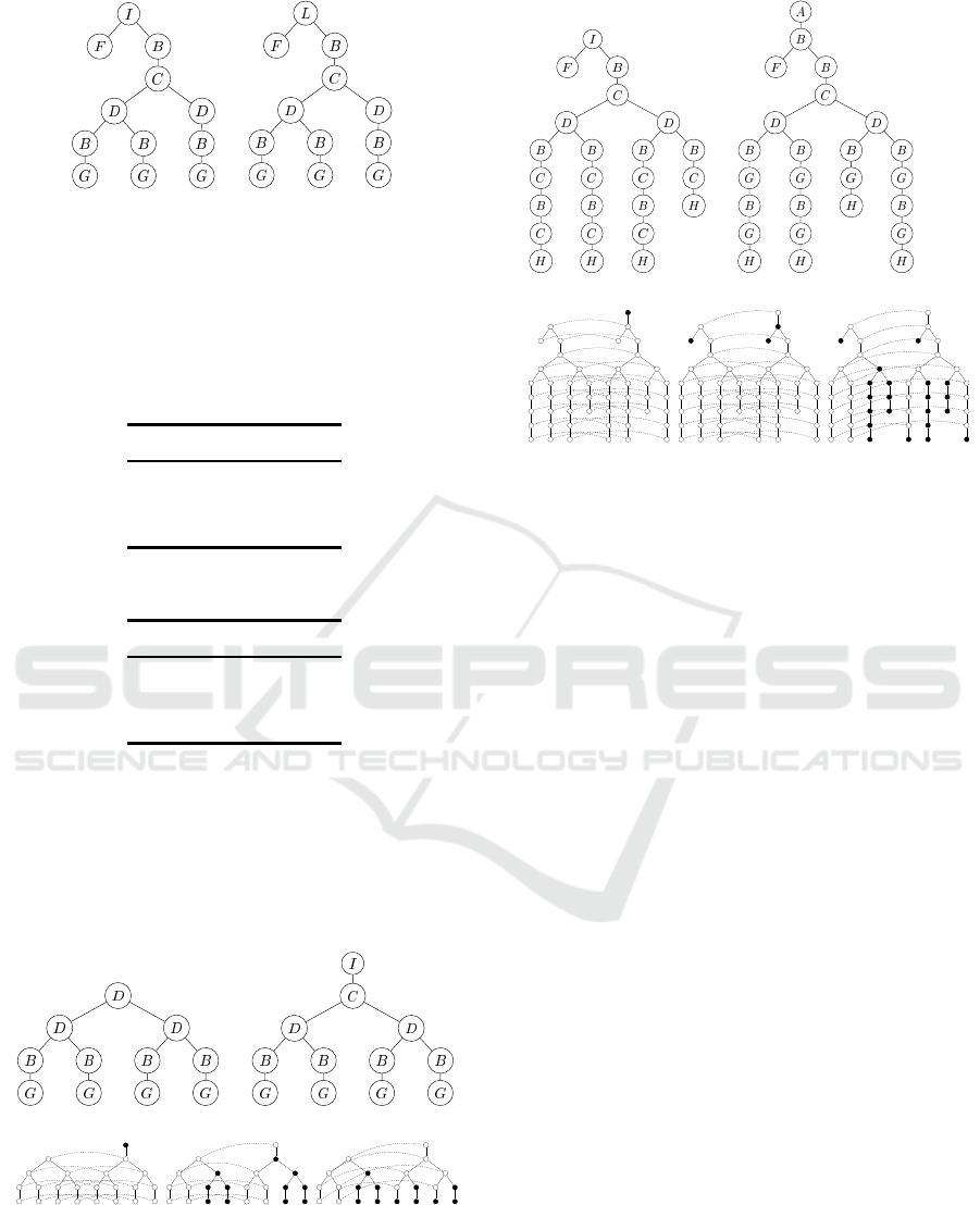
Example 1. Consider trees T

and T

illustra-

ted in Figure 5, that is, one tree (T

) is obtai-

ned by deleting leaves to another tree (T

). In

this case, it holds that τ

) ≤ EMD

For the trees T

and T

in Figure 5, it holds that

) = 1 and EMD

) = 1.357 for every

A ∈ {ILST, ACC, LCA, LCART, TOP}.

It is obvious that τ

) = 1. On the ot-

her hand, it holds that τ

],T

]) = 1 and

],T

]) = |T

]| (1 ≤ i ≤ 6). Since the

weight of T

] (resp., T

]) is 1/6 (resp., 1/7), the

optimum ﬂow consists of the 6 ﬂows from T

] to

] whose costs are 1/7 and the 6 ﬂows from T

]

to T

] whose costs are 1/42. Then, the cost of the

optimum ﬂow is 6(1/7)+(6+5+4+3+2+1)/ 42 =

57/42 = 1.357 = EMD

Hence, wherea s the ground distance s are not sen-

sitive to inserting leaves, the EMD is necessary to

transport th e remained weig hts for every node in one

tree to an inserted leave in an other tree.

= G01687 T

= G02836

Figure 5: Trees T

and T

Example 2. Consider trees T

and T

illustrated in

Figure 6, th at is, just a label of the root in one tree

) is different from that in another tree (T

). In

this case, it holds that EMD

) ≤ τ

For the trees T

and T

in Figure 6, it holds that

) = 1 and EMD

) = 0.083 for every

A ∈ {ILST, ACC, LCA, LCART, TOP}.

It is obvious that τ

) = 1. On the other

hand, the signature containing r(T

) (resp., r(T

)) is

just T

(resp., T

) itself. Since τ

],T

]) = 0

for 2 ≤ i ≤ 12, the cost of the ﬂow from T

] to T

]

is 0. Since the weight of T

] and T

] is 1/12 and

],T

]) = 1, the cost of the optimum ﬂow is

1/12 + 11(0/12) = 0.083 = EMD

Hence, the difference near to the root is more sen-

sitive to the ground distances rather than the EMDs.

Furthermore, in this case, th e E MDs is much smaller

than the ground distance.

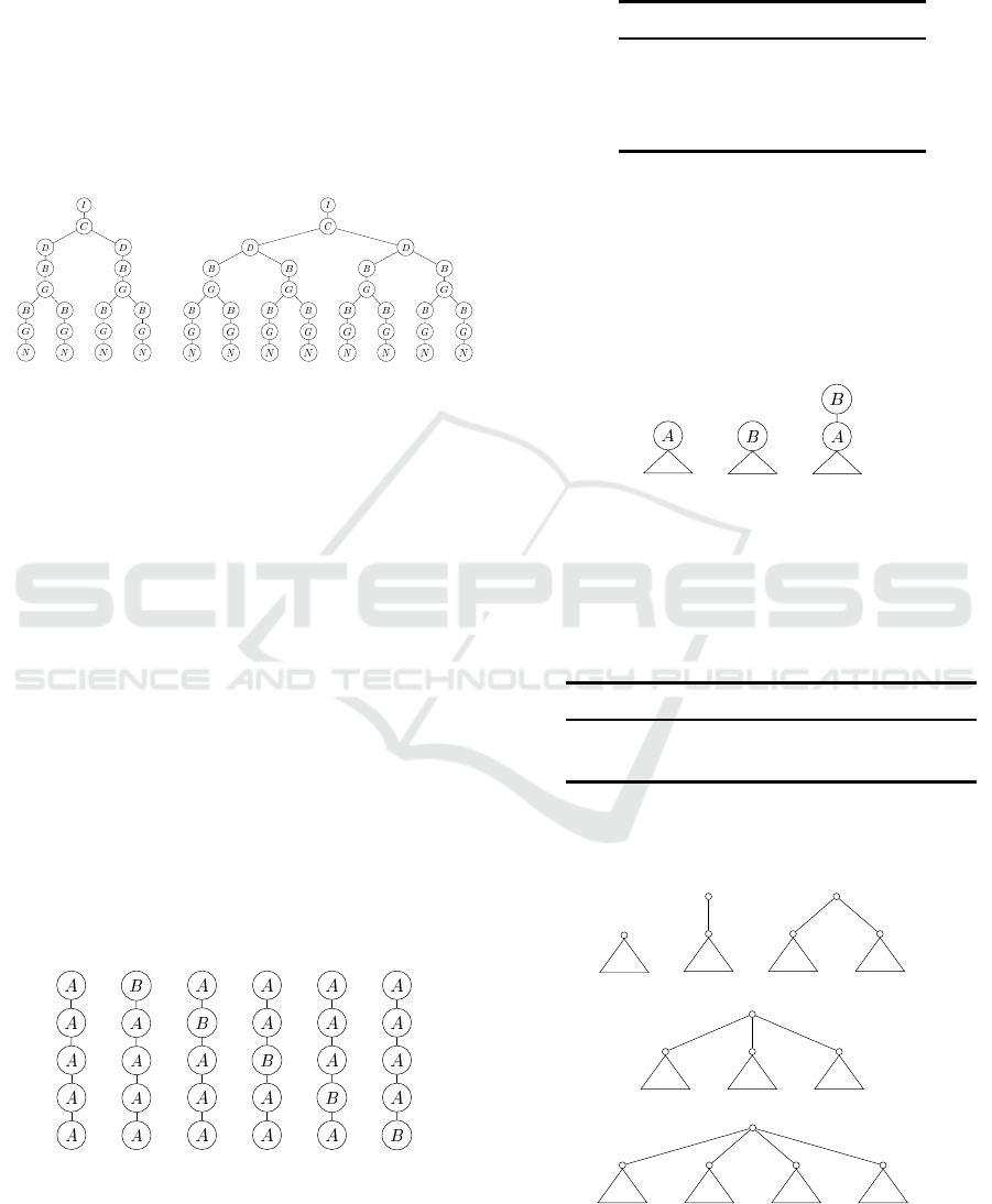
Example 3. Consider trees T

and T

illustrated in

Figure 7 and T

and T

illustrated in Figure 8, that

Earth Mover’s Distances for Rooted Labaled Unordered Trees based on Tai Mapping Hierarchy

165

= G00340 T

= G01413

Figure 6: Trees T

and T

is, one tree (T

or T

) is obtained by deleting the

root of another tree ( T

or T

). For these cases,

it holds that EMD

LCART

) ≤ τ

LCART

) and

EMD

TOP

) ≤ τ

TOP

). For the trees T

and

in Figure 7, τ

) and EMD

) are:

A τ

EMD

LCA 2 0.841

LCART 12 0.91 7

TOP 17 1.512

For the tre es T

and T

in Figure 8, τ

) and

EMD

) are:

A τ

EMD

LCA 2 0.810

LCART 4 0.813

TOP 34 1.092

Here, we also illustrate the minimum cost map-

ping in M

in Figures 7 and 8, where the correspon-

ding node is denoted by ◦ and the non-corresponding

node is denoted by •, which implies τ

The reason is that the structural difference near to

the root is much sensitive to τ

LCART

and τ

TOP

, whose

values tend to be large, but th e EMDs are not.

= G00449 T

= G00513

LCA

) M

LCART

) M

TOP

)

Figure 7: Trees T

and T

Example 4. Consider trees T

and T

illustrated in

Figure 9, that is, subtrees in one tree (T

) frequently

occur in another tree (T

). In this case, it holds

= G03673 T

= G04688

LCA

) M

LCART

) M

TOP

)

Figure 8: Trees T

and T

that EMD

) is much smaller than τ

For the trees T

and T

in Figure 6, it holds that

) = 16 and EMD

) = 1.63 for every

A ∈ {ILST, ACC, LCA, LCART, TOP}. Since T

obtained by inserting 16 nodes to T

, it holds that

) = 16.

The weight of T

[u] (resp., T

[v]) is 1/20 (resp.,

1/36). Then, T

], T

]

and T

] are isomorphic an d T

], T

] and T

] are isomorphic, so the we ights of

], T

] and T

] as features are 2/20,

4/36, 4/20 and 8/36, respectively. Since these weig-

hts are preser ved in the su btrees of them, the total

weight of features consisting of T

] and its sub -

trees in T

is 2/20 +2/20 +4/20+4/20= 16/20 and

that of T

] and its subtrees in T

is 4/36 + 4/36 +

8/36 + 8/36 = 32/36. Hence, the cost of ﬂows in

these isomorphic subtree s from T

to T

is 0, be-

cause τ

],T

]) = 0, for example. Since these

ﬂows move all the weight 16/ 20 of T

], T

] and

its subtrees can receive the weight 32/36 − 16/20 =

4/45.

For the remained featu res in T

, the weights of

], T

] and T

] as features are 1/36, 1/36

and 2/36, respectively. Furthermore, as T

] and its

subtrees receive the weights, it is necessary to con-

sider the ground distances between T

] and T

]

(4 ≤ i ≤ 8). The ground distances necessary to com-

pute EMD

) are given as follows.

ICPRAM 2018 - 7th International Conference on Pattern Recognition Applications and Methods

166

],T

]) = 16, τ

],T

]) = 16,

],T

]) = 8, τ

],T

]) = 3,

],T

]) = 4, τ

],T

]) = 1,

],T

]) = 2, τ

],T

]) = 6,

],T

]) = 7, τ

],T

]) = 8.

Hence, by computing the optimum ﬂow to re ceive

the weight 4/ 45 + 4/36 = 1/5 in T

, we can o btain

EMD

) as 16(1/ 36) + 16(1/36) + 8(1/90) +

3(1/45)+ 4 (1/45) + 1(1/90) +2(1/90)+ 6(1/45) +

7(1/45) + 8(1/45) = 49/30 = 1.633.

= G03824 T

= G04045

Figure 9: Trees T

and T

4.4 Properties of EMDs for Trees

Finally, we investigate the properties of the EMDs for

trees by summarizing the typical c ases in Section 4 .3.

1. Concerned with Example 1, just the case that one

tree is obtained by deleting leaves to another tree

implies th at τ

) ≤ EMD

) for N-

glycan data. Whereas the trees T

and T

in Ex-

ample 1 are paths, the statement holds when some

internal nodes have some leaves as children.

As another case concerned with Example 1, con-

sider trees T

(1 ≤ i ≤ 6) in Figure 10. Then, it

holds that τ

) = 1 for every i (2 ≤ i ≤ 6)

but EMD

) = 0.2, EMD

) = 0.4,

EMD

) = 0.6, EMD

) = 0.8 and

EMD

) = 1. The reason is that the farther

node with a different label from the root makes

more different signatures.

Figure 10: Trees T

(1 ≤ i ≤ 6).

2. Concerned with Examples 2 and 3, consider

complete binary trees T

and T

with 15 no-

des and a tree T

adding the root to T

illustra-

ted in Figure 11. Then, for A ∈ {ILST, TOP},

EMD

) and τ

) are as follows.

EMD

ILST

) 0.067 0.796

EMD

TOP

) 0.067 1.07

ILST

) 1 1

TOP

) 1 23

Hence, the difference of bo th labels and structu -

res near to the root is more sensitive to τ

TOP

than

EMD

TOP

. On the other hand, for the difference

of labels near to the root, EMD

is much smal-

ler than τ

. As stated in Examples 2 and 3, there

also exists a case that LCATOP is sensitive to the

difference of both labels a nd structures nea r to the

root.

Figure 11: Trees T

, T

and T

3. Co ncerned with Example 4, co nsider a tree T

with 10 nodes and trees T

(2 ≤ i ≤ 5) contai-

ning T

as subtrees illustrated in Figure 12. Then ,

EMD

) and τ

) are as follows.

EMD

) 0.5 0.738 0.822 0.866

) 1 11 21 31

In this case, whereas the ground distances are ne-

cessary to insert new nodes, the EMDs tend to ab-

sorb the inﬂuence of isomorphic subtrees.

Figure 12: Trees T

(1 ≤ i ≤ 5).

Earth Mover’s Distances for Rooted Labaled Unordered Trees based on Tai Mapping Hierarchy

167

5 CONCLUSION

In this paper, for the variations of edit distance τ

for

A ∈ {ILST, ACC, LCA, LCART, TOP}, we have for-

mulated the earth mover’s distances EMD

based on

. Then, we have given experimental results to eva-

luate EMD

comparing with τ

. As a result, we have

investigated the properties of EMD

It is a future work to give experimental results for

more large data (with large degrees) to analyze the

theoretical ratio O(n logn/d) in Section 4.1 in expe-

rimental. Also it is a future work to formulate EMDs

to other tra c ta ble variations in Tai mapping hierar-

chy (Yoshino and Hirata, 2017).

Concerned w ith Ex ample 1 in Section 4.3 and Ste-

tement 1 in Section 4. 4, we have found no trees T

and T

such that τ

) < EMD

) except

the case that T

is obtained by deleting leaves to T

Then, it is a fu ture work to determine whether or

not there exist other cases satisfying that τ

) <

EMD

It is a future work to analyze the properties of

EMDs in Section 4.4 in more detail and investigate

how data are appropriate for EMDs. In particular,

since it is possible that the number of the signature is

too small to formulate EMDs for trees, it is an impor-

tant future work to investigate appropriate signatures

for EMDs for trees.

ACKNOWLEDGEMENTS

This work is partially supported by Grant-in-

Aid for Scientiﬁc Research 17H00762, 16H02870,

16H01743 and 15K12102 fro m the Ministry of Edu-

cation, Cu lture, Sports, Science and Te chnology, Ja-

pan.

REFERENCES

Aratsu, T., Hirata, K., and Kuboyama, T. (2009). Sibling

distance for rooted labeled trees. In JSAI PAK DD ’08

Post-Workshop Proc. (LNAI 5433), pages 99–110.

Chawathe, S. S. (1999). Comparing hierarchical data in ex-

ternal memory. In Proc. VLDB’99, pages 90–101.

Gollapudi, S. and Panigrahy, R. (2008). The power of two

min-hashes for similarity search among hierarchical

data objects. In Proc. PODS’08, pages 211–219.

Hirata, K., Yamamoto, Y., and Kuboyama, T. (2011). Im-

proved MAX SNP-hard results for ﬁnding an edit dis-

tance between unordered trees. In Proc. CPM’11

(LNCS 6661), pages 402–415.

Jiang, T., Wang, L., and Z hang, K. (1995). Al ignment of

trees – an alternative to tree edit. Theoret. Comput.

Sci., 143:137–148.

Kailing, K., Kriegel, H.-P., Sch¨onaur, S., and Seidl, T.

(2004). Efﬁcient simi larity search for hierarchical data

in large databases. In Proc. EDBT’04, pages 676–693.

Kawaguchi, T. and Hirata, K. (2017). On earth mover’s

distance based on complete subtrees for rooted labeled

trees. In Proc. SISA’17, pages 225–228.

Kuboyama, T. (2007). Matching and learning in trees. Ph.D

thesis, University of Tokyo.

Li, F., Wang, H., Li, J., and Gao, H. (2013). A survey on

tree edit distance lower bound estimation techniques

for similarity join on XML data. SIGMOD Record,

43:29–39.

Luke, S. and Panait, L. (2001). A survey and comparison

of tree generation algorithms. In Proc. GECCO’01,

pages 81–88.

Rubner, Y., Tomasi, C., and Guibas, L. J. (2007). The earth

mover’s distance as a metric for image retrieval. Int.

J. Comput. Visi on, 40:99–121.

Selkow, S. M. (1977). The tree-to-tree editing problem. In-

form. Process. Lett., 6:184–186.

Tai, K.-C. (1979). The tree-to-tree correction problem. J.

ACM, 26:422–433.

Yamamoto, Y., Hirata, K., and Kuboyama, T. (2014). Trac-

table and intractable variations of unordered tree edit

distance. Internat. J. Found. Comput. Sci., 25:307–

329.

Yoshino, T. and Hirata, K. ( 2017). Tai mapping hierarchy

for rooted labeled trees through common subforest.

Theory of Comput. Sys., 60:769–787.

Zhang, K. (1995). Algorithms for t he constrained edi-

ting distance between ordered labeled trees and related

problems. Pattern Recog., 28:463–474.

Zhang, K. (1996). A constrained edit distance between

unordered labeled trees. Algorithmica, 15:205–222.

Zhang, K. and Jiang, T. ( 1994). Some MAX SNP-hard re-

sults concerning unordered labeled trees. Inform. Pro-

cess. Lett., 49:249–254.

Zhang, K., Wang, J., and Shasha, D. (1996). On the editing

distance between undirected acyclic graphs. I nternat.

J. Found. Comput. Sci., 7:43–58.

ICPRAM 2018 - 7th International Conference on Pattern Recognition Applications and Methods

168