
Dynamic Multiscale Tree Learning using Ensemble Strong Classifiers for
Multi-label Segmentation of Medical Images with Lesions
Samya Amiri
1,2
, Mohamed Ali Mahjoub
2
and Islem Rekik
3
1
Isitcom - Higher Institute of Computer Science and Communication Techniques of Hammam Sousse,
University of Sousse, Tunisia
2
LATIS lab, ENISo – National Engineering School of Sousse, University of Sousse, Tunisia
3
BASIRA lab, CVIP Group, School of Science and Engineering, Computing, University of Dundee, U.K.
Keywords:
Ensemble Classifiers, Dynamic Learning, Autocontext Model, Structured Random Forest, Bayesian Network,
Brain Tumor Segmentation, MRI.
Abstract:
We introduce a dynamic multiscale tree (DMT) architecture that learns how to leverage the strengths of dif-
ferent state-of-the-art classifiers for supervised multi-label image segmentation. Unlike previous works that
simply aggregate or cascade classifiers for addressing image segmentation and labeling tasks, we propose to
embed strong classifiers into a tree structure that allows bi-directional flow of information between its classi-
fier nodes to gradually improve their performances. Our DMT is a generic classification model that inherently
embeds different cascades of classifiers while enhancing learning transfer between them to boost up their clas-
sification accuracies. Specifically, each node in our DMT can nest a Structured Random Forest (SRF) classifier
or a Bayesian Network (BN) classifier. The proposed SRF-BN DMT architecture has several appealing pro-
perties. First, while SRF operates at a patch-level (regular image region), BN operates at the super-pixel level
(irregular image region), thereby enabling the DMT to integrate multi-level image knowledge in the learning
process. Second, the proposed DMT robustly overcomes the limitations of the aggregated classifiers through
the ascending and descending flow of contextual information between each parent node and its children nodes.
Third, we train DMT using different scales to capture a coarse-to-fine image details. Last, DMT demonstrates
its outperformance in comparison to several state-of-the-art segmentation methods for multi-labeling of brain
images with gliomas.
1 INTRODUCTION
Accurate multi-label image segmentation is one of
the top challenges in both computer vision and me-
dical image analysis. Specifically, in computer-aided
healthcare applications, medical image segmentation
constitutes a critical step for tracking the evolution of
anatomical structures and lesions in the brain using
neuroimaging, as well as quantitatively measuring
group structural difference between image populati-
ons (Havaei et al., 2017; Valverde et al., 2017; Christ
et al., 2017; Wang et al., 2016; Loic et al., 2016).
Multi-label image segmentation is widely addressed
as a classification problem. Previous works (Li et al.,
2004; Wei et al., 2014) used individual classifiers such
as support vector machine (SVM) to segment each
label class independently, then fuse the different la-
bel maps into a multi-label map. However, prior to
the fusion step, the produced label maps may largely
overlap one another, which might yield to biased fu-
sed label map. Alternatively, the integration of multi-
ple classifiers within the same segmentation frame-
work would help reduce this bias and improve the
overall multi-label classification performance since M
heads are better than one as reported in (Lee et al.,
2015). Broadly, one can categorize the segmenta-
tion methods that combine multiple classifiers into
two groups:(1) cascaded classifiers, and(2) ensem-
ble classifiers. In the first group, classifiers are chai-
ned such that the output of each classifier is fed into
the next classifier in the cascade to generate the final
segmentation result at the end of the cascade. Such
architecture can be adopted for two different goals.
First, cascaded classifiers take into account contex-
tual information, encoded in the segmentation map
outputted from the previous classifier, thereby enfor-
cing spatial consistency between neighboring image
elements (e.g., patches, superpixels) in the spirit of an
auto-context model (Havaei et al., 2017; Qian et al.,
2016; Zhang et al., 2016b; Loic et al., 2016). Se-
Amiri, S., Mahjoub, M. and Rekik, I.
Dynamic Multiscale Tree Learning using Ensemble Strong Classifiers for Multi-label Segmentation of Medical Images with Lesions.
DOI: 10.5220/0006630004190426
In Proceedings of the 13th International Joint Conference on Computer Vision, Imaging and Computer Graphics Theory and Applications (VISIGRAPP 2018) - Volume 4: VISAPP, pages
419-426
ISBN: 978-989-758-290-5
Copyright © 2018 by SCITEPRESS – Science and Technology Publications, Lda. All rights reserved
419
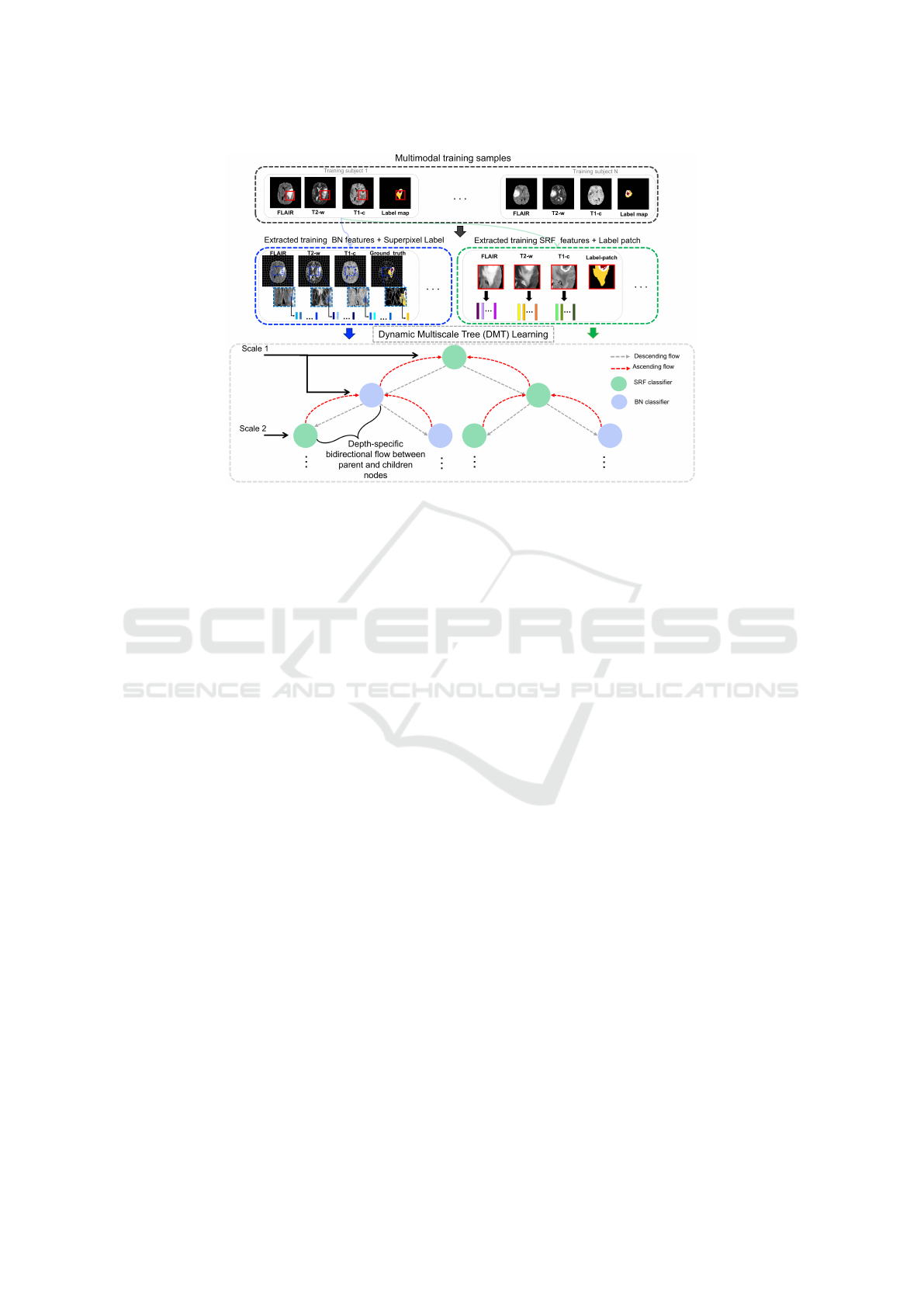
Figure 1: Proposed Dynamic Multi-scale Tree (DMT) learning architecture for multi-label classification (training stage).
DMT embeds SRF and BN classifiers into a binary tree architecture, where a depth-specific bidirectional flow occurs between
parent and children nodes making the tree learning dynamic. During training, SRF learns a mapping between feature patches
extracted from three MRI modalities and their corresponding label patches for each training subject; whereas, BN classifier
learns conditional probabilities from the superpixels of the oversegmented multimodal MR images and the label map.
cond, this allows to combine classifiers hierarchically,
where each classifier in the cascade is assigned to a
more specific segmentation task (or a sub-task), as
it further sub-labels the output label map of its an-
tecedent classifier (Dai et al., 2016; Valverde et al.,
2017; Christ et al., 2017; Wang et al., 2016). Alt-
hough these methods produced promising results, and
clearly outperformed the use of single (non-cascaded)
classifiers in different image segmentation applicati-
ons, cascading classifiers only allows a unidirectio-
nal learning transfer, where the learned mapping from
the previous classifier is somehow communicated’ to
the next classifier in the chain for instance through
the output segmentation map. The second group re-
presents ensemble classifiers based methods, which
train individual classifiers, then aggregate their seg-
mentation results (Rahman and Tasnim, 2014). Spe-
cifically, such frameworks combine a set of indepen-
dently trained classifiers on the same labeling pro-
blem and generates the final segmentation result by
fusing the individual segmentation results using a fu-
sion method, which is typically weighted or unweig-
hted voting (Kim et al., 2015). Hence, it constructs
a strong classifier that outperforms each individual
‘weak’ classifier (or base classifier) (Lee et al., 2015).
For instance, Random Forest (RF) classification algo-
rithm, independently trains weak decision trees using
bootstrap samples generated from the training data
to learn a mapping between the feature and the la-
bel sets (Breiman, 2001). The segmentation map of a
new input image is the aggregation of the trees’ de-
cisions by major voting. RF demonstrated its effi-
ciency in solving different image classification pro-
blems (Qian et al., 2016; Zhang et al., 2016b), which
reflects the power of the ensemble classifiers techni-
que. In addition to significantly improving the seg-
mentation results when compared with single classi-
fiers, ensemble classifiers based methods are powerful
in addressing several known classification problems
such as imbalanced correlation and over-fitting (Yi-
jing et al., 2016). However, such combination techni-
que is not enough to fully exploit the training of clas-
sifiers and leverage their strengths. Indeed, the base
classifiers perform segmentation independently wit-
hout any cooperation to solve the target classification
problem. Moreover, the learning of each classifier in
the ensemble is performed in one-step, as opposed to
multi-step classifier training, where the learning of
each classifier gradually improves from one step to
the next one. We note that this differs from cascaded
classifiers, where each classifier is visited’ or trained
once through combining the contextual segmentation
map of the previous classifier along with the original
input image.
To address the aforementioned limitations of both
categories, we propose a Dynamic Multi-scale Tree
(DMT) architecture for multi-label image segmenta-
tion. DMT is a binary tree, where each node nests
a classifier, and each traversed path from the root
node to a leaf node encodes a cascade of classifiers
VISAPP 2018 - International Conference on Computer Vision Theory and Applications
420

(i.e., nodes on the path). Our proposed DMT archi-
tecture allows a bidirectional information flow bet-
ween two successive nodes in the tree (from parent
node to child node and from child node back to parent
node). Thus, DMT is based on ascending and des-
cending feedbacks between each parent node and its
children nodes. This allows to gradually refine the le-
arning of each node classifier, while benefitting from
the learning of its immediate neighboring nodes. To
generate the final segmentation results, we combine
the elementary segmentation results produced at the
leaf nodes using majority voting strategy. The pro-
posed architecture integrates different possible com-
binations of different classifiers, while taking advan-
tage of their strengths and overcoming their limita-
tions through the bidirectional learning transfer bet-
ween them, which defines the dynamic aspect of the
proposed architecture. Furthermore, the DMT inhe-
rently integrates contextual information in the classi-
fication task, since each classifier inputs the segmen-
tation result of its parent node or children nodes clas-
sifiers. Additionally, to capture a coarse-to-fine image
details for accurate segmentation, the DMT is desig-
ned to consider different scale at each level in the tree
in a way that the adopted scale decreases as we go
deeper along the tree edges nearing its leaf nodes.
In this work, we define our DMT classifica-
tion model using two strong classifiers: Structured
Random Forest (SRF) and Bayesian Network (BN).
SRF is an improved version of Random Forest (Kont-
schieder et al., 2011). In addition of being fast, resis-
tant to over-fitting and having a good performance in
classifying high-dimensional data, SRF handles struc-
tural information and integrates spatial information.
It has shown good performance in several classifica-
tion tasks especially muli-label image segmentation
(Kontschieder et al., 2011; Zhang et al., 2016a). On
the other hand, BN is a learning graphical model that
statistically represents the dependencies between the
image elements and their features. It is suitable for
multi-label segmentation for its effectiveness in fu-
sing complex relationships between image features
of different natures and handling noisy as well as
missing signals in images (Zhang and Ji, 2008; Pa-
nagiotakis et al., 2011; Zhang and Ji, 2011; Yang
et al., 2015). Embedding SRF and BN within our
DMT leverages their strengths and helps overcome
their limitations (i.e. not accurately classifying transi-
tions between label classes for SRF and the problem
of parameters learning such as prior probabilities for
BN). Moreover, the SRF-BN bidirectional coopera-
tion during learning and testing stages enables the in-
tegration of multi-level image knowledge through the
combination of regular and irregular image elements
(i.e. patch-level classification produced by SRF and
superpixel-level classification produced by BN). To
sum up, our SRF-BN DMT has promise for multi-
label image segmentation as it:
• Gradually improves the classification accuracy
through the bidirectional flow between parents
and children nodes, each nesting a BN or SRF
classifier
• Simultaneously integrates multi-level and multi-
scale knowledge from training images, thereby
examining in depth the different inherent image
characteristics
• Overcomes SRF and BN limitations when used
independently through multiple cascades (or tree
paths) composed of different combinations of BN
and SRF classifiers.
2 BASE CLASSIFIERS
In this section we briefly introduce the SRF and BN
classifiers, that are embedded as nodes in our DMT
classification framework. Then,we explain in detail
how we define our DMT architecture.
2.1 Structured Random Forest
SRF is a variant of the traditional Random Forest clas-
sifier, which better handles and preserves the structure
of different labels in the image (Kontschieder et al.,
2011). While, standard RF maps an intensity feature
vector extracted from a 2D patch centered at pixel x
to the label of its center pixel x (i.e., patch-to-pixel
mapping), SRF maps the intensity feature vector to
a 2D label patch centered at x (patch-to-patch map-
ping). This is achieved at each node in the SRF tree,
where the function that splits patch features between
right and left children nodes depends on the joint dis-
tribution of two labels: a first label at the patch cen-
ter and a second label selected at a random position
within the training patch (Kontschieder et al., 2011).
We also note that in SRF, both feature space and label
space nest patches that might have different dimensi-
ons. Despite its elegant and solid mathematical foun-
dation as well as its improved performance in image
segmentation compared with RF, SRF might perform
poorly at irregular boundaries between different label
classes since it is trained using regularly structured
patches (Kontschieder et al., 2011). Besides, it does
not include contextual information to enforce spatial
consistency between neighboring label patches. To
address these limitations, we first propose to embed
SRF as a classifier node into our DMT architecture,
Dynamic Multiscale Tree Learning using Ensemble Strong Classifiers for Multi-label Segmentation of Medical Images with Lesions
421

where the contextual information is provided as a seg-
mentation map by its parent and children nodes. Se-
cond, we improve its training around irregular boun-
daries through leveraging the strength of one or more
its neighboring BN classifiers, which learns to seg-
ment the image at the superpixel level, thereby better
capturing irregular boundaries in the image.
2.2 Bayesian Network
Various BN-based models have been proposed for
image segmentation (Zhang and Ji, 2008; Panagiota-
kis et al., 2011; Zhang and Ji, 2011). In our work,
we adopt the BN architecture proposed in (Zhang and
Ji, 2011). As a preprocessing step, we first generate
the edge maps from the input MR image modalities
Fig1. This edge map consists of a set of superpixels
S
p
i
;i = 1 ...N (or regional blobs) and edge segments
E
j
; j = 1...L.
We define our BN as a four-layer network, where
each node in the first layer stores a superpixel. The se-
cond layer is composed of nodes, each storing a single
edge from the edge map. The two remaining layers
store the extracted superpixel features and edge featu-
res, respectively. During the training stage, to set BN
parameters, we define the prior probability P(S
p
i
) of
S
p
i
as a uniform distribution and then learn the con-
ditional probability representing the relationship be-
tween the superpixels’ features and their correspon-
ding labels using a mixture of Gaussians model. In
addition, we empirically define the conditional pro-
bability modeling the relationship between each su-
perpixel label and each edge state (i.e., true or false
edge) P(E
j
|p
a
(E
j
)), where p
a
(E
j
) denotes the parent
superpixel nodes of E
j
.
During the testing stage, we learn the BN struc-
ture through encoding the semantic relationships be-
tween superpixels and edge segments. Specifically,
each edge node has for parent nodes the two super-
pixel nodes that are separated by this edge. In other
words, each superpixel provides contextual informa-
tion to judge whether the edge is on the object boun-
dary or not. If two superpixels have different labels,
it is more likely that there is a true object boundary
between them, i.e. E
j
= 1, otherwise E
j
= 0 .
Although automatic segmentation methods based
on BN have shown great results in the state-of-the-
art, they might perform poorly in segmenting low-
contrast image regions and different regions with si-
milar features (Zhang and Ji, 2011). To further im-
prove the segmentation accuracy of BN, we propose
to include additional information through embedding
BN classifier into the DMT learning architecture.
3 PROPOSED MULTI-SCALE
DYNAMIC TREE LEARNING
In this section, we present the main steps in devi-
sing our Multi-scale Dynamic Tree segmentation fra-
mework, which aims to boost up the performance of
classifiers nested in its nodes. Fig1 illustrates the pro-
posed binary tree architecture composed of classifier
nodes, where each classifier ultimately communica-
tes the output of its learning (i.e., semantic context
or probability segmentation maps) to its parent and
children nodes. Therefore, the learning of the tree is
dynamic as it is based on ascending and descending
feedbacks between each parent node and its child-
ren nodes. Specifically, each node output is fed to
the children nodes as semantic context, in turn the
children nodes transfer their learning (i.e. probabi-
lity maps) to their common parent node. Then, af-
ter merging these transferred probability maps from
children nodes, the parent node uses the merged maps
as a contextual information to generate a new segmen-
tation result that will be subsequently communicated
again to its children nodes. This gradually improves
the learning of its classifier nodes at each depth level
of the tree. In the following sections, we further detail
the DMT architecture.
3.1 Dynamic Tree Learning
We define a binary tree T(V,E), where V denotes the
set of nodes in T and E represents the set of edges in
T. Each node i in T represents a classifier c
i
and each
edge e
i j
connecting two nodes i and j carries bidirecti-
onal contextual information flow between the classi-
fiers c
i
and c
j
that are always inputting the original
image characteristics (i.e. the features for SRF, su-
perpixel features and input image edge map for BN).
Specifically, we define bidirectional feedbacks bet-
ween two neighboring classifier nodes i and j, enco-
ding two flows: a descending flow F
i→ j
that repre-
sents the transfer of the probability maps generated
by parent classifier node c
i
to its child classifier node
c
j
as contextual information and an ascending flow
F
j→i
that models the transfer of the probability maps
generated by a child node c
j
back to its parent node c
i
(Fig. 2). This depth-wise bidirectional learning trans-
fer occurs locally along each edge between a parent
node and its child node, thereby defining the dyna-
mics of the tree.
In addition, as our Dynamic Tree (DT) grows ex-
ponentially, it integrates various combinations of clas-
sifiers. Thus, each path of the tree implements a uni-
que cascade of classifiers. To generate the final seg-
mentation result we aggregate the segmentation maps
VISAPP 2018 - International Conference on Computer Vision Theory and Applications
422

Figure 2: Implicit and explicitlearning transfer in the propo-
sed dynamic multi-scale tree-based classification architec-
ture. The dashed gray arrows denote the descending flows
from the parent classifier c
i
to its children c
j
and c
0
j
(itera-
tion k), while the dashed red arrows denote the ascending
flows derived from the children nodes to their parent node.
Both ascending flows are fused for the parent node to inte-
grate them in generating a new segmentation map that will
be communicated to its two children classifier nodes (itera-
tion k +1).
produced at each leaf node in the binary tree by ap-
plying the majority voting.
Inherent Implicit and Explicit Transfer Learning
between Nodes in DT Architecture. We note that
the bidirectional flow between parent nodes and their
corresponding children nodes defines a new traver-
sing strategy of the tree nodes, that in addition to the
dynamic learning aspect, encodes two different types
of learning transfer: explicit and implicit. Indeed, the
ascending and descending flows between parent no-
des and their children through the direct transfer of
their generated probability maps is an explicit lear-
ning transfer. However, in our binary tree, when a
parent node i receives the ascending flows (F
k
( j → i)
and F
k
( j
0
→ i) from its left and right children nodes j
and j’, they are fused before being passed on, in a se-
cond round, as contextual information (F
k+1
(i → j)
and F
k+1
(i → j
0
)) to the children nodes (Fig. 2). The
probability maps fusion at the parent node level is per-
formed through simple averaging. In particular, the
parent node concatenates the fused probability map
with the original input features to generate a new seg-
mentation probability map result that will be commu-
nicated to its two children classifier nodes. Hence,
the children nodes of the same parent node explicitly
cooperate to improve their parent learning, and impli-
citly cooperate to improve their own learning while
using their parent node as a proxy.
SRF-BN Dynamic Tree. In this work, each classi-
fier node is assigned a SRF or a BN model, previ-
ously described in Section 2, to define our Dynamic
Tree architecture. The transferred information bet-
ween classifiers through the descending and ascen-
ding flows is used in addition to the testing image
features as contextual information, while BN classi-
fier uses this information as prior knowledge (i.e prior
probability) to perform the multi-label segmentation
task. The combination of SRF and BN classifiers is
compelling for the following reasons. First, it en-
hances the performance of BN by taking the poste-
rior probability generated by SRF as prior probability.
This justifies our choice of the root node of our DT as
a SRF. Second, it improves SRF performance around
irregular between-class boundaries since SRF benefits
from BN structure learning, which is based on image
over-segmentation that is guided by object bounda-
ries. Third, as the SRF maps image information at the
patch level, while BN models knowledge at the super-
pixel level, their combination allows the aggregation
of regular (i.e. patch) and irregular (i.e. superpixel)
structures in the image for our target multi-label seg-
mentation task.
3.2 Dynamic Multi-scale Tree Learning
To further boost the performance of our multi-label
segmentation framework and enhance the segmen-
tation accuracy, we introduce a multi-scale learning
strategy in our dynamic tree architecture by varying
the size of the input patches and superpixels used to
grow the SRF and construct the BN classifier. Spe-
cifically, we use a different scale at each depth level
such as we go deeper along the tree edges nearing its
leaf nodes, we progressively decrease the size of both
patches and superpixels in the training and testing sta-
ges. In addition to capturing coarse-to-fine details of
the image anatomical structure, the application of the
multi-scale strategy to the proposed DT allows to cap-
ture fine-to-coarse information. Indeed, DMT lear-
ning semantically divides the image into different pat-
terns (e.g., different patches and superpixels at each
depth of the tree) in both intensity and label domains
at different scales. However, thanks to the bidirectio-
nal dynamic flow, the scale defined at each depth in-
fluences the performance of parent nodes (in previous
level) and children nodes (in next level), which allows
to simultaneously perform coarse-to-fine and fine-to-
coarse information integration in the multi-label clas-
sification task. Moreover, a depth-wise multi-scale
feature representation adaptively encodes image fe-
atures at different scales for each image pixel in the
image element (superpixel or patch).
3.3 Statistical Superpixel-based and
Patch-based Feature Extraction
To train each classifier node in the tree, we extract
the following statistical features at the superpixel le-
Dynamic Multiscale Tree Learning using Ensemble Strong Classifiers for Multi-label Segmentation of Medical Images with Lesions
423

vel (for BN) and 2D patch level (for SRF): first or-
der operators; higher order operators, texture features,
and spatial context features (Prastawa et al., 2004).
4 RESULTS AND DISCUSSION
Dataset and Parameters. We evaluate our proposed
brain tumor segmentation framework on 50 subjects
with high-grade gliomas, randomly selected from the
Brain Tumor Image Segmentation Challenge (BRATS
2015) dataset (Menze et al., 2015). For each patient,
we use three MRI modalities (FLAIR, T2-w, T1-c) al-
ong with the corresponding manually segmented gli-
oma lesions.
For the baseline methods training we adopt the
following parameters:(1) Edgemap generation: we
use the SLIC oversegmentation algorithm with a su-
perpixel number fixed to 1000 and compactness fixed
to 10 (Achanta et al., 2010). To establish superpixel-
to-superpixel correspondence across modalities for
each subject, we first oversegment the FLAIR MRI,
then we apply the generated edgemap (i.e., superpixel
partition) to the corresponding T1-c and T2-w MR
images. (2) SRF training: we grow 15 trees using
intensity feature patches of size 10x10 and label pat-
ches of size 7x7. (3) BN construction: the BN model
is built using the generated edgemap as detailed in
Section 2; the conditional probabilities modeling the
relationships between the superpixel labeling and the
edge state are defined as follows: P(E
j
= 1|p
a
(E
j
)) =
0.8 if the parent region nodes have different labels and
0.2 otherwise.
Evaluation and Comparison Methods. For com-
parison, as baseline methods we use: (1) SRF: the
Random Forest version that exploits structural infor-
mation described in Section 2, (2) BN: the classifica-
tion algorithm described in Section 2 where the prior
probability of superpixels is set as a uniform distri-
bution, (3) SRF-SRF denotes the auto-context Struc-
tured Random Forest, (4) BN-BN denotes the auto-
context Bayesian Network, where the first BN prior
probability is set as a uniform distribution while the
second classifier use the posterior probability of its
previous as prior probability. Of note, by conventio-
nal auto-context classifier, we mean a uni-directional
contextual flow from one classifier to the next one.
The segmentation frameworks were trained using
leave-one-patient cross-validation experiments. For
evaluation, we use the Dice score between the ground
truth region area A
gt
and the segmented region area A
s
as follows D = (A
gt
T
A
s
)/2(A
gt
+ A
s
).
Next, we investigate the influence of the tree depth
as well as the multi-scale tree learning strategy on the
performance of the proposed architecture.
Varying Tree Architectures. In this experiment, we
evaluate two different tree architectures to examine
the impact of the tree depth on the framework per-
formance. Table. 1 shows the segmentation results
for 2-level tree (i.e. depth=2) and 1-level tree (i.e.
depth=1) for tumor lesion multi-label segmentation
with and without multiscale variant. Although the
average Dice Score has improved from depth 1 to 2,
the improvement wasn’t statistically significant. We
did not explore larger depths (d¿2), since as the binary
tree grows exponentially, its computational time dra-
matically increases and becomes demanding in terms
of resources (especially memory).
Multi-scale Tree Architecture. To examine the in-
fluence of the multiscale DT learning strategy, we
compare the conventional DT architecture (at a fixed-
scale) to MDT architecture. For the fixed-scale ar-
chitecture, all tree nodes nest either an SRF classifier
trained using intensity feature patches of size 10x10
and label patches of size 7x7 or a BN classifier con-
structed using an edgemap of 1000 superpixels gene-
rated with a compactness of 10. In the multiscale ar-
chitecture, we keep the same parameters of the fixed-
scale architecture at the first level of the tree while the
classifiers of the second level are trained with diffe-
rent parameters. Specifically, we use smaller inten-
sity patches (of size 8x8) and label patches (of size
5x5) for the SRF training, and a smaller number of
superpixels for BN construction (1200 superpixels).
Clearly, the quantitative results show the outper-
formance (improvement of 7%) of both proposed DT
and DMT architectures in comparison with several
baseline methods for multi-label tumor lesion seg-
mentation with statistical significance (p ≺ 0.05) .
This indicates that a deeper combination of diffe-
rent learning models helps increase the segmentation
accuracy. When comparing the results of the SRF and
BN we found that SRF outperforms BN in segmenting
the three classes: wHole Tumor (HT), Core Tumor
(CT) and Enhancing Tumor (ET) Table. 1 . This is
due to the fact that BN have difficulties in segmenting
low-contrast images and identifying different super-
pixels having similar characteristics, especially with
the lack of any prior knowledge on the anatomical
structure of the testing image. Although BN has a
low Dice score compared to SRF, in Fig. 3 we can
note that it has better performance in detecting the
boundaries between different classes. This shows the
impact of the irregular structure of superpixels used
during BN training and testing, which gives BN the
ability to be more accurate in detecting object boun-
daries compared to SRF that considers regular image
patches. Notably, BN structure is individualized du-
VISAPP 2018 - International Conference on Computer Vision Theory and Applications
424
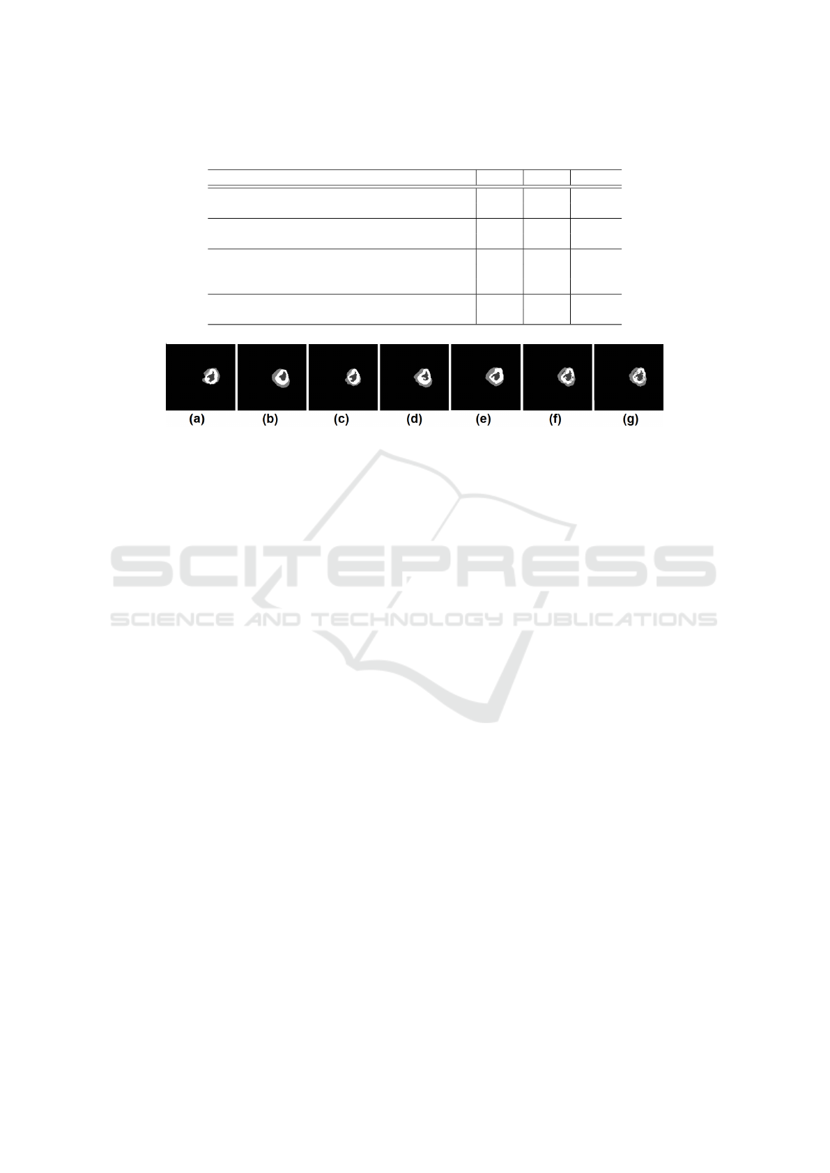
Table 1: Segmentation results of the proposed framework and comparison methods averaged across 50 patients. (HT: whole
Tumor; CT: Core Tumor; ET: Enhanced Tumor; depth of the tree; * indicates outperformed methods with p − value ≺ 0.05).
Methods HT CT ET
Dynamic Multiscale Tree-Learning (depth =2) 89.64 82.3 80
Dynamic Multiscale Tree-Learning (depth =1) 88.93 79.7 78.09
Dynamic Tree-Learning (depth =2) 89.56 80.43 79
Dynamic Tree-Learning (depth =1) 88.07 78.7 77.94
SRF-BN 82.5 72.6 70
SRF-SRF 80 70.05 37.12
BN-BN 79.82 71 56. 14
SRF 75 60 35
BN 70.8 45 32
Figure 3: Qualitative segmentation results for all the baseline methods: (a) BN segmentation result. (b) SRF segmentation
result. (c) Auto-context BN. (d) Auto-context SRF. (e) SRF+BN segmentation result. (f) DMT segmentation result. (depth=2).
(g) Ground truth label map.
ring the testing stage for each testing subject since it
is based on the testing image oversegmentation map.
Thus, SRF and BN classifiers are complementary.
First, they perform segmentation at regular and irre-
gular structures of the image. Second, one (SRF) le-
arns image knowledge during the training stage, while
the other (BN) is structured using the input testing
image during the testing stage through modeling the
testing image structure. Further, the results of SRF-
SRF and BN-BN models that implement the auto-
context approach show an improvement of the seg-
mentation results at both qualitative and quantitative
levels when compared with baseline SRF and BN mo-
dels. More importantly, we note that BN-BN cascade
outperforms SRF-SRF cascade when segmenting the
Core Tumor and Enhancing Tumor (ET) lesions. This
can be explained by the fine and irregular anatomi-
cal details of these image structures when compa-
red to the whole tumor lesion. Since BN is trained
using irregular superpixels, it produced more accurate
segmentation for these classes (e.g., BN-BN:56.14 vs
SRF-SRF: 37.12 for ET). Through further cascading
both SRF and BN classifiers, we note that the hetero-
geneous SRF-BN cascade produced much better re-
sults compared to both autocontext SRF and autocon-
text BN for two main reasons. First SRF aids in defi-
ning BN prior based on the testing image structure,
while BN enhances the performance of SRF at the
boundaries level. This further highlights the impor-
tance of integrating both regular and irregular image
elements for training classifiers that capture different
image structures. The outperformance of the propo-
sed DMT architecture also lays ground for our as-
sumption that embedding SRF and BN into our uni-
fied dynamic architecture where they mutually benefit
from their learning boosts up the multi-label segmen-
tation accuracy. In addition to the previously menti-
oned advantages of combining SRF and BN, it is im-
portant to note that the integration of variant cascades
of SRF and BN endows our architecture with an effi-
cient learning ability.
5 CONCLUSIONS
We proposed a Dynamic Multi-scale Tree (DMT) le-
arning architecture that both cascades and aggregates
classifiers for multi-label medical image segmenta-
tion. Specifically, our DMT embeds classifiers into a
binary tree architecture, where each node nests a clas-
sifier and each edge encodes a learning transfer bet-
ween the classifiers. A new tree traversal strategy is
proposed where a depth-wise bidirectional feedbacks
are performed along each edge between a parent node
and its child node. This allows explicit learning bet-
ween parent and children nodes and implicit learning
transfer between children of the same parent. Moreo-
ver, we train DMT using different scales for input pat-
ches and superpixels to capture a coarse-to-fine image
details as well as a fine-to-coarse image structures
through the depth-wise bidirectional flow. In our fu-
ture work, we will devise a more comprehensive tree
traversal strategy.
Dynamic Multiscale Tree Learning using Ensemble Strong Classifiers for Multi-label Segmentation of Medical Images with Lesions
425

REFERENCES
Achanta, R., Shaji, A., Smith, K., Lucchi, A., Fua, P., and
S
¨
usstrunk, S. (2010). Slic superpixels. Technical re-
port.
Breiman, L. (2001). Random forests. Machine learning,
45(1):5–32.
Christ, P. F., Ettlinger, F., Gr
¨
un, F., Elshaera, M. E. A., Lip-
kova, J., Schlecht, S., Ahmaddy, F., Tatavarty, S., Bic-
kel, M., Bilic, P., et al. (2017). Automatic liver and
tumor segmentation of ct and mri volumes using cas-
caded fully convolutional neural networks. arXiv pre-
print arXiv:1702.05970.
Dai, J., He, K., and Sun, J. (2016). Instance-aware semantic
segmentation via multi-task network cascades. In Pro-
ceedings of the IEEE Conference on Computer Vision
and Pattern Recognition, pages 3150–3158.
Havaei, M., Davy, A., Warde-Farley, D., Biard, A., Cour-
ville, A., Bengio, Y., Pal, C., Jodoin, P.-M., and
Larochelle, H. (2017). Brain tumor segmentation
with deep neural networks. Medical image analysis,
35:18–31.
Kim, H., Thiagarajan, J., Jayaraman, J., and Bremer, P.-
T. (2015). A randomized ensemble approach to in-
dustrial ct segmentation. In Proceedings of the IEEE
International Conference on Computer Vision, pages
1707–1715.
Kontschieder, P., Bulo, S. R., Bischof, H., and Pelillo, M.
(2011). Structured class-labels in random forests for
semantic image labelling. In Computer Vision (ICCV),
2011 IEEE International Conference on, pages 2190–
2197. IEEE.
Lee, S., Purushwalkam, S., Cogswell, M., Crandall, D., and
Batra, D. (2015). Why m heads are better than one:
Training a diverse ensemble of deep networks. arXiv
preprint arXiv:1511.06314.
Li, X., Wang, L., and Sung, E. (2004). Multilabel svm
active learning for image classification. In Image
Processing, 2004. ICIP’04. 2004 International Con-
ference on, volume 4, pages 2207–2210. IEEE.
Loic, L. F., Aditya, V. N., Javier, A.-V., Richard, L., and
Antonio, C. (2016). Segmentation of brain tumors via
cascades of lifted decision forests. In Proceedings of
BRATS Challenge-MICCAI.
Menze, B. H., Jakab, A., Bauer, S., Kalpathy-Cramer, J.,
Farahani, K., Kirby, J., Burren, Y., Porz, N., Slot-
boom, J., Wiest, R., et al. (2015). The multimodal
brain tumor image segmentation benchmark (brats).
IEEE transactions on medical imaging, 34(10):1993–
2024.
Panagiotakis, C., Grinias, I., and Tziritas, G. (2011). Na-
tural image segmentation based on tree equipartition,
bayesian flooding and region merging. IEEE Tran-
sactions on Image Processing, 20(8):2276–2287.
Prastawa, M., Bullitt, E., Ho, S., and Gerig, G. (2004). A
brain tumor segmentation framework based on outlier
detection. Medical image analysis, 8(3):275–283.
Qian, C., Wang, L., Gao, Y., Yousuf, A., Yang, X., Oto, A.,
and Shen, D. (2016). In vivo mri based prostate can-
cer localization with random forests and auto-context
model. Computerized Medical Imaging and Graphics,
52:44–57.
Rahman, A. and Tasnim, S. (2014). Ensemble classi-
fiers and their applications: A review. arXiv preprint
arXiv:1404.4088.
Valverde, S., Cabezas, M., Roura, E., Gonz
´
alez-Vill
`
a, S.,
Pareto, D., Vilanova, J.-C., Rami
´
o-Torrent
`
a, L., Ro-
vira,
`
A., Oliver, A., and Llad
´
o, X. (2017). Improving
automated multiple sclerosis lesion segmentation with
a cascaded 3d convolutional neural network approach.
arXiv preprint arXiv:1702.04869.
Wang, L., Pedersen, P., Agu, E., Strong, D., and Tulu, B.
(2016). Area determination of diabetic foot ulcer ima-
ges using a cascaded two-stage svm based classifica-
tion. IEEE Transactions on Biomedical Engineering.
Wei, Y., Xia, W., Huang, J., Ni, B., Dong, J., Zhao, Y., and
Yan, S. (2014). Cnn: Single-label to multi-label. arXiv
preprint arXiv:1406.5726.
Yang, S., Yuan, C., Wu, B., Hu, W., and Wang, F. (2015).
Multi-feature max-margin hierarchical bayesian mo-
del for action recognition. In Proceedings of the IEEE
Conference on Computer Vision and Pattern Recogni-
tion, pages 1610–1618.
Yijing, L., Haixiang, G., Xiao, L., Yanan, L., and Jin-
ling, L. (2016). Adapted ensemble classification algo-
rithm based on multiple classifier system and feature
selection for classifying multi-class imbalanced data.
Knowledge-Based Systems, 94:88–104.
Zhang, J., Gao, Y., Park, S. H., Zong, X., Lin, W., and Shen,
D. (2016a). Segmentation of perivascular spaces using
vascular features and structured random forest from
7t mr image. In International Workshop on Machine
Learning in Medical Imaging, pages 61–68. Springer.
Zhang, L. and Ji, Q. (2008). Integration of multiple contex-
tual information for image segmentation using a baye-
sian network. In Computer Vision and Pattern Recog-
nition Workshops, 2008. CVPRW’08. IEEE Computer
Society Conference on, pages 1–6. IEEE.
Zhang, L. and Ji, Q. (2011). A bayesian network model for
automatic and interactive image segmentation. IEEE
Transactions on Image Processing, 20(9):2582–2593.
Zhang, L., Wang, Q., Gao, Y., Li, H., Wu, G., and Shen,
D. (2016b). Concatenated spatially-localized random
forests for hippocampus labeling in adult and infant
mr brain images. Neurocomputing.
VISAPP 2018 - International Conference on Computer Vision Theory and Applications
426
