
Layered Graph Force-driven Vertex Positioning
Radek Ma
ˇ
r
´
ık
Faculty of Electrical Engineering, Czech Technical University, Technicka 2, Prague, Czech Republic
Keywords:
Force-driven Layout, Layered Graph, Multitree, Spanning Tree, Phylogenetic Network, Genealogical
Network.
Abstract:
We propose a new method of node positioning for huge layered graphs specified by layers and fixed ordering
of nodes within layers. We assume that the assignments of nodes to the layers and the order of nodes within
the layers are provided by other suitable methods capable of processing multitree like networks. The node
positioning method is based on the force-driven approach with barrier-like repulsive forces that avoids the
quadratic complexity of traditional methods. We demonstrate achievements on several datasets containing
up to millions of people or species. The proposed layout method of layered graphs that are close to acyclic
multitrees creates aesthetically acceptable layouts in linear time.
1 INTRODUCTION
Although it has been more than 55 years since Tutte
introduced barycentric embedding, research of graph
visualization techniques remains a highly active field
attracting much attention (Tutte, 1963). Working with
tree-like structures such as genealogical or phyloge-
netic networks is no exception in this sense. We will
use a genealogical graph as an exemplar of general
tree-like networks to simplify our further discussion.
Applications to other tree-like network domains are
provided in the section dedicated to experiments.
In many situations the resulting network layout is
produced by state of the art tools as required (a brief
overview of such tools is provided in Section 2). Nev-
ertheless, the tools can often only process networks
up to several thousand nodes. The tools and methods
that are able to cope with millions of nodes and edges
are not able to cover additional constraints, such as
the layering of node children into the same layer and
keeping the order of nodes within a given layer as ex-
pected in genealogical network visualizations.
In this paper, we propose a new node positioning
method that keeps both assignments of nodes to layers
and the order of nodes within each layer. The method
is very fast and therefore can operate with networks
having more than a million nodes and edges. The
method is based on the force-driven approach with
barrier-like repulsive forces that avoids the quadratic
complexity of traditional methods.
Thus, in this paper we focus on the third most
critical aspect discussed by Sugiyama in (Sugiyama
et al., 1981), also related to the third step of the main
algorithm proposed in (Gansner et al., 1993), node
positioning:
1. determination of generations (layers, node ranks),
2. enforcing node orders within the layers,
3. setting the actual layout coordinates of nodes
(node positioning),
4. design of edges.
In other words, we assume that node layers and or-
ders in the layers are fixed in an optimal way (they
should not be changed) and it is necessary to accom-
plish only node positioning. The rest of the steps,
such as layering and ordering, is performed by other
methods able to operate within huge networks, e.g.
such as those proposed for multitree-close networks
in (Marik, 2017).
The remainder of the paper is organized in the fol-
lowing way. In the next section, a brief overview
of related tools and methods is given. Then in Sec-
tion 3, we provide a summary of important mathe-
matical concepts used in this paper. We continue with
a description of the proposed method’s technical de-
tails and its steps in Section 4. Finally, we discuss
achieved results tested on datasets with up to millions
of nodes in Section 5.
2 RELATED METHODS
In the following paragraphs, we provide a brief
overview of the methods related to the method pro-
posed in this article. Sections 2.1 and 2.2 review
Ma
ˇ
rík, R.
Layered Graph Force-driven Vertex Positioning.
DOI: 10.5220/0006624703010308
In Proceedings of the 13th International Joint Conference on Computer Vision, Imaging and Computer Graphics Theory and Applications (VISIGRAPP 2018) - Volume 3: IVAPP, pages
301-308
ISBN: 978-989-758-289-9
Copyright © 2018 by SCITEPRESS – Science and Technology Publications, Lda. All rights reserved
301

methods related to layering and ordering that serve
as preprocessing steps to node positioning. Having
this context established, node positioning methods are
then described in Section 2.3.
2.1 Multitree Close Networks Layering
and Node Ordering
Tree based drawing methods for phyloge-
netic/genealogical graphs have been one of the
standard techniques for centuries. Ancestor trees,
descendant trees and Hourglass charts are part
of the traditional tools employed by the major-
ity of freeware, shareware, or commercial tools,
for example Gramps (Gramps, 2016), MyHer-
itage (MyHeritage, 2016), TreePlus (Lee et al.,
2006), GraphViz (Gansner and North, 2000), and
Phylo.io (Robinson et al., 2016). There are also
other more space-efficient representations such as
fan charts or H-charts (Tuttle et al., 2010; Kieffer
et al., 2016). As any pure tree representation enables
any ordering of node predecessors/successors, it is
possible to specify the type of ordering, such as
children ordered by their birth dates. Furthermore,
tree representations can be laid out in such a way that
family members are grouped together. The tools are
not able to process huge networks, which are not pure
trees, with millions of nodes while still satisfying
constraints on node layering and ordering.
However, the situation with family member
grouping changes significantly if the assumptions of
one main person and direct ancestors/descendants are
dropped. In a number of cases, it is highly ben-
eficial if the entire network of families, or at least
a significant part, can be displayed in one layout.
Then we often deal with structures close to multitrees
and face difficult issues linked with edge crossing
and preferences on node clustering (Warfield, 1977;
Sugiyama et al., 1981) with occasional cycles usu-
ally caused by mistakes in datasets. Therefore, the
standard techniques for planar graph layouts (Lem-
pel et al., 1967; Hopcroft and Tarjan, 1974; Shih and
Hsu, 1999) including planarization techniques (Re-
sende and Ribeiro, 2001; Chimani et al., 2008) are
not suitable in all cases because of a higher than lin-
ear complexity.
As we assume multitree-like networks, we would
like to stress the significance of layers, so we con-
sider a layout design targeting layered drawing (Healy
and Nikolov, 2013). A layering and ordering method
targeting huge tree-close networks with up to several
millions of nodes that ensures some node layer and
order constraints was introduced in (Marik, 2017). A
two-level approach when a given quasi-tree (a graph
having O(|V |) biconnected components) is decom-
posed into a tree of biconnected components where
biconnected components are drawn with a force-
directed approach with subtrees placed onto concen-
tric rings was proposed in (Archambault et al., 2006).
Both approaches (Archambault et al., 2006; Marik,
2017) use a spanning tree to drive the high level lay-
out, but they differ in optimization criteria. The ma-
jority of algorithms for node layering are derived from
the topological order computation, O(|V | + |E|) time
complexity (Cormen et al., 2009).
2.2 Constrained Graph Layout
There is also a class of methods that tackle graph
layout while satisfying different types of constraints
targeting, for example, node separation, drawing cy-
cles, and non-overlapping clusters (Dwyer and Koren,
2005; Dwyer, 2009). Although the methods are ap-
plicable to more general networks than those close to
multitree treated in this paper, they have a higher com-
plexity (often quadratic) than linear. The experiments
presented networks of up to 10,000 nodes only. The
given node layers and the order of nodes within layers
assumed in this paper can be expressed using about
O(|V |
2
) node separation constraints that leads to an
unfeasible problem for networks with the number of
nodes of magnitude |V | ≈ 10
6
.
2.3 Node Positioning
In this paper, we assume that layers of nodes and
a node order within the layers are given and fixed.
Therefore, we focus only on a new node positioning
force-driven method. At first, we refer to the tradi-
tional reference by Tutte (Tutte, 1963). His paper
focuses mainly on 3-connected planar graphs. Tutte
considered barycentric graph embedding. The paper
is also referenced as the first “force-directed” algo-
rithm because suitable vertex positions can be found
by solving a system of linear equations, so that it
exhibits features of force-directed methods (Battista
et al., 1999). Sugiyama in (Sugiyama et al., 1981)
proposed vertex positions calculated using quadratic
programming with an objective function combining
distances among vertices from neighboring layers and
distances from lower and upper layer barycenters that
is minimized. In 1984, Eades (Eades, 1984) intro-
duced the spring-embedder model in which graph ver-
tices are denoted by a set of rings, each pair of rings
is connected by a spring and the spring is associated
with two types of forces: attraction forces and repul-
sive forces. Fruchterman and Reingold (Fruchterman
and Reingold, 1991) added the even vertex distribu-
IVAPP 2018 - International Conference on Information Visualization Theory and Applications
302
tion criterion to the previous two, aiming for the same
length of edges and a layout symmetry and also exper-
imented with a number of force forms. They selected
a model in which nodes at a distance d are attracted
to each other by the attractive force f
a
following the
quadratic form and they are pushed apart by the re-
pulsive force f
r
f
a
(d) = d
2
/k, f
r
(d) = −k/d
2
, (1)
where k is the optimal distance between vertices de-
fined as
k = C
r
area
|V |
(2)
Both algorithms (Eades, 1984) and (Fruchterman and
Reingold, 1991) compute attractive forces between
adjacent vertices and repulsive forces between all
pairs of vertices. Thus, these classical algorithms ex-
hibit a quadratic complexity and do not keep a given
node ordering. We will propose a suitable modifica-
tion of the force-directed method to position ordered
nodes in layers in almost linear time.
3 TREE-LIKE NETWORKS
To begin, we need to demarcate the structures we
treat in this paper. We aim for domain data that
cannot be modeled as pure tree structures. We as-
sume directed tree-like networks that can form hier-
archies, occasionally exhibit sharing of subtrees, and
ones in which strongly connected components very
rarely occur. We do not attempt to assess to which
level such a structure deviates from a tree although
we are aware of some quantification methods (Doro-
govtsev and Mendes, 2003; Gu and Sun, 2010). We
follow the usual graph theory terminology (Diestel,
2005; Bondy and Murty, 2008).
A layering L = (L
1
,L
2
,. ..,L
h
) of a graph, G =
(V,E) is an ordered partition of V into non-empty lay-
ers L
i
such that adjacent vertices are in different lay-
ers, i.e. if {u,v} ∈ E, where u ∈ L
i
and v ∈ L
j
, then
i 6= j (Brandes and K
¨
opf, 2002). An ordering of a
layered graph is a partial order ≺ of V such that either
u ≺ v or v ≺ u if and only if L(u) = L(v).
4 NODE POSITIONING
We assume that the partitions of the vertices into lay-
ers and node orders in each graph layer are precom-
puted and fixed, e.g. by a method in (Marik, 2017)
following the first two phases proposed by Sugiyama.
The order of nodes in layers is the main force driv-
ing the resulting graph layout. However, there is still
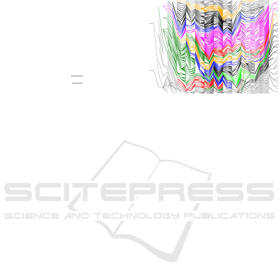
Figure 1: A private family tree (Mykiska’s network). A
visualization of a sample private family tree with 2192 indi-
viduals and 765 marriages created using the uniform spac-
ing method. The layout is created very quickly (below 0.5
second with a Python script on DELL XPS 13 using an In-
tel i7 2GHz processor). The visualization demonstrates the
unpleasant zig-zag layout that might be difficult to read for
large networks. The layers are drawn vertically from left to
right.
a large number of possibilities in which to assign 2D
coordinates to the nodes. In the following paragraphs
we discuss and propose two techniques for node po-
sition calculations that also satisfy the constraints on
node orders. As the order of nodes in layers can be
determined in O(|V |) time for multitree-like networks
we focus only on techniques that scale in a similar
way. All the following methods assume that graph
layers are placed uniformly in a horizontal direction.
Additionally, the nodes are linked with straight-lined
edges.
We start with a simple positioning technique that
produces results that might not be easily readable. It is
based on uniform spacing. Then, we provide a tech-
nique inspired by force-directed methods. We show
that there is a combination of special attractive and
repulsive forces that enables the readjustment of node
positions quickly, even for millions of nodes.
4.1 Uniform Spacing
A very simple technique is based on uniform spacing.
Nodes in each graph layer are placed with a uniform
distance in a vertical direction. A layout generated us-
ing the ordering method proposed in the paper (Marik,
2017) and using uniform node spreading in both di-
rections is shown in Fig 1. Family clans (subtrees
of the undirected spanning tree of the processed net-
work) with more than 150 nodes in presented visual-
izations are emphasized by different colors. An ideal
layout would result in edges creating colored horizon-
Layered Graph Force-driven Vertex Positioning
303

tal strips with only a minimum number of crossings.
Rapid zig-zag changes (waves) in color strips in verti-
cal directions make graph reading more difficult. On
the other hand, the computation can be performed in
linear time O(|V |) and it provides a kind of top-level
overview for very large graphs with millions of nodes.
4.2 Force-directed Node Positioning
Although node ordering based on uniform spacing
produces useable results for very large graph data, its
zig-zag form makes reading difficult. Another method
we have investigated is based on force-directed node
positioning.
We assume again that nodes are layered and or-
dered within layers. Therefore, we need a method that
is capable of reducing the wavy format while retain-
ing the order of nodes in layers.
Force-directed node positioning uses two types of
forces: attractive and repulsive ones. Our goal is to
make waves straight so we define attractive forces be-
tween nodes linked by edges and belonging to differ-
ent layers. Thus, attractive forces push linked nodes
to each other which in turn decreases the range of
the zig-zag wavy form of strips (subtrees). We use
attractive forces following the quadratic form intro-
duced by Fruchterman and Reingold (Fruchterman
and Reingold, 1991), see Equation (1). We also need
to use repulsive forces to keep vertices apart. We
propose a local barrier-like force instead of f
r
(d) ac-
cording to Equation (1) leading to the quadratic com-
plexity. The resulting force for each node must hold
the node ordering and the two node separation con-
straints. Forces are applied iteratively while nodes
move significantly.
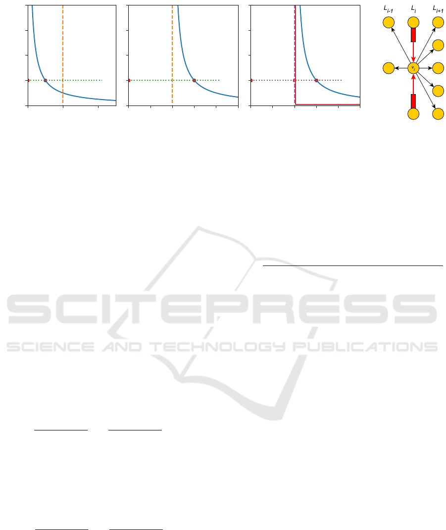
The diagram in Figure 2(d) depicts forces
schematically. Both types of forces are projected in
the direction along a given layer (a vertical in our
case). The optimum distance k is defined as a dis-
tance of nodes in a layer with the largest number of
nodes L
max
if the nodes are placed uniformly, i.e.
k = δ = C/|L
max
|, C is the predefined height of the
layout. If the actual definition of the forces is taken as
proposed in (Fruchterman and Reingold, 1991) then
the actual distance of nodes might converge to a very
small fraction of δ because there are only one or two
sources of the repulsion. In addition, a number of
neighboring nodes can generate attraction in one di-
rection and the nodes are prescribed to stay in the
same order. The variant a) in Figure 2 captures an
instance in which the vertices v
i
and v
i+1
in the same
layer are pushed so close to each other that the to-
tal sum of all projected attractive forces f
a
i
shown as
a given value and pulling the vertex v
i
is in equilib-
rium with the repulsive force f
r
i
generated by the ver-
tex v
i+1
. In real layouts the resulting distance of both
vertices might be a tiny fraction of the minimum sepa-
ration constraint δ. A modification of repulsive forces
compensating such cases can be defined to generate
an infinite repulsive force at distance δ by shifting
the repulsive force field beyond the minimum sepa-
ration distance as is shown in variant b). However,
in both cases, displacements of nodes in each itera-
tion become very small after a few iterations and then
the algorithm converges very slowly. The repulsive
force from the neighbors of a given node is necessary
to propagate forces through the network in order to
reach their equilibrium.
However, there is another way to propagate re-
pulsive forces. We can imagine a repulsive force
with a profile in which a repulsive force between
two neighbor nodes v
(i)
j
,v
(i)
k
∈ L
i
is 0 if their distance
d
jk
= |x(v
k
) − x(v
j
)| ≥ δ and ∞ if d
jk
< δ. In other
words, such a profile models a barrier at distance δ,
see Figure 2 variant c). If d
jk
< δ, we say that the
barrier between v
j
and v
k
is active. While this vari-
ant of repulsive force reflects the shifted modification
discussed above, case b), it cannot be easily used for
force propagation. Nevertheless, having neighboring
nodes in the layer order, we can approximate the re-
pulsive force of a given node by the attractive forces
of its neighboring nodes if their barriers are active.
In fact, we only consider the two direct neighboring
nodes in the rest of the paper.
We will show that if repulsive forces are modeled
as barriers then the problem leads to a solution com-
bining barycenters of vertex clusters that can be per-
formed iteratively again in linear time. In fact, repul-
sive forces are modeled as decision procedures realiz-
ing barriers. In each iteration, each node is moved to
its equilibrium position or the nearest barrier if such a
position is not reachable.
As vertices are strictly tied to a given layer, we
can only focus on projections of forces towards the
direction of the layer. Thus, we can denote the union
of the lower and upper neighbors of the given vertex
v as N
v
= N
−
v
∪ N
+
v
. Furthermore, we drop the upper
index of the k layer in the following steps for vertices
v
i
= v
(k)
i
∈ L
k
with the exception of v
j
∈ N
v
i
. The coor-
dinate of vertex v
i
will be denoted as x
i
= x(v
i
). Let f
a
i
be a total attractive force pulling the vertex v
i
and hav-
ing the quadratic form f
a
i
(x
i
) = 1/δ
∑
v
j
∈N
v
i
(x
j
− x
i
)
2
.
The optimum position µ
I
i
= arg min
x
i
f
a
i
of the vertex
v
i
can be found as an minimum of the function f
a
i
us-
ing
d f
a
i
dx
i
!
= 0. Thus, the resulting equilibrium position
µ
I
i
= 1/|N
v
i
|
∑
v
j
∈N
v
i
x
j
(3)
IVAPP 2018 - International Conference on Information Visualization Theory and Applications
304
0
δ
1.0
f
r
i
v
i
v
i+1
f
a
i
(a)
0
δ
v
i
v
i+1
f
a
i
(b)
0
δ
distance
v
i
v
i+1
f
a
i
v
i
v
i+1
f
a
i
(c) (d)
Figure 2: Repulsive force variants. Three different variants of repulsive force models. Nodes v
i
and v
i+1
of the same layer
mark the resulting position of v
i+1
relatively to the position of v
i
. f
r
i
is the sum of all repulsive forces. a) The variant
proposed by Fruchterman and Reingold breaking the minimum separation δ constraint. b) Its shifted modification satisfying
the minimum separation constraint. c) The barrier variant proposed and used in this article. d) Forces on a vertex. Attractive
(black) forces from the lower and upper vertex neighbors pull the vertex v
i
towards their barycentric position. Repulsive (red)
forces from the vertex predecessor and successor in the layer L
i
push the vertex v
i
away to maintain the minimum separation
constraint δ. The vertices might be equipped by a solid separation barrier schematically drawn as red rectangles. Only force
projections to the layer L
i
need to be treated because of the layer constraint.
is the barycentric position of v
i
. The vertex v
i
should
be placed into the equilibrium position µ
I
i
if no barrier
to the predecessor v
i−1
or the successor v
i+1
is active.
If a barrier is active then we need to combine two or
three force sources as we have a node and at most two
of its neighbor barriers active. Let us assume that the
active barrier is between the vertex v
i
and its succes-
sor v
i+1
. The position of v
i
is x
i
and the position of
v
i+1
is x
i+1
= x
i
+ δ. The total attractive force f
a
i+1
pulling the successor v
i+1
pushes also the vertex v
i
as
the repulsive force. Thus, if only this one barrier is
active, then the total force pulling the vertex v
i
is
f
Is
i
(x
i
) = f
a
i
(x
i
) + f
a
i+1
(x
i+1
) = f
a
i
(x
i
) + f
a
i+1
(x
i
+ δ)
(4)
In this case equilibrium can be reached at the position
µ
Is
i
=
|N
v
i
|
|N
v
i
| + |N
v
i+1
|
µ
I
i
+
|N
v
i
+1
|
|N
v
i
| + |N
v
i+1
|
(µ
I
i+1
− δ)
(5)
In other words, the equilibrium position µ
Is
i
is a con-
vex combination of no barrier equilibrium positions
with the successor displaced by −δ. Similarly, we
can obtain the equilibrium position of v
i
, only if the
barrier with the predecessor is active
µ
pI
i
=
|N
v
i
|
|N
v
i
| + |N
v
i−1
|
µ
I
i
+
|N
v
i
−1
|
|N
v
i
| + |N
v
i−1
|
(µ
I
i−1
+ δ)
(6)
If both the barriers with the predecessor and the suc-
cessor are active, we start with the total force pulling
the vertex v
i
f
pIs
i
(x
i
) = f
a
i−1
(x
i−1
) + f
a
i
(x
i
) + f
a
i+1
(x
i+1
) = (7)
= f
a
i−1
(x
i
− δ) + f
a
i
(x
i
) + f
a
i+1
(x
i
+ δ) (8)
for which the equilibrium position of the vertex v
i
is
µ
pIs
i
=
|N
v
i
−1
|(µ
I
i−1
+ δ) + |N
v
i
|µ
I
i
+ |N
v
i
+1
|(µ
I
i+1
− δ)
|N
v
i−1
| + |N
v
i
| + |N
v
i+1
|
(9)
Furthermore, we need to determine what case of ac-
tive barriers occurs to calculate the new optimum po-
sition x
0
i
of the vertex v
i
. This can be accomplished
using a simple decision procedure:
1. if µ
I
i−1
≤ µ
I
i
− δ and µ
I
i
+ δ ≤ µ
I
i+1
, then x
0
i
:= µ
I
i
;
2. if µ
I
i−1
> µ
I
i
− δ and µ
pI
i
+ δ ≤ µ
I
i+1
, then x
0
i
:= µ
pI
i
;
3. if µ
I
i−1
≤ µ
Is
i
− δ and µ
I
i
+ δ > µ
I
i+1
, then x
0
i
:= µ
Is
i
;
4. otherwise x
0
i
:= µ
pIs
i
.
We update the vertices positions layer by layer fol-
lowing the order of vertices in the given layer. We
perform two such sweeps in the forward direction and
then two sweeps in the backward direction (both lay-
ers and orders) to speed up node position changes
propagation. The initial positions of vertices are de-
termined using the uniform spacing strategy. As we
move only one node, although its new position is the
result of all its neighboring nodes, we also need to
satisfy the order of vertices. We again use another de-
cision procedure to determine a new feasible position
x
00
i
for the vertex v
i
1. if x
0
i
≤ x
i−1
+ δ then x
00
i
:= x
i−1
+ δ,
2. if x
0
i
≥ x
i+1
− δ then x
00
i
:= x
i+1
− δ,
3. otherwise x
00
i
:= x
0
i
.
The new feasible positions might result in position os-
cillations. Thus, the new position x
?
i
of the vertex
Layered Graph Force-driven Vertex Positioning
305

Table 1: Sample datasets and their basic network statistics: a node number |V | of the complete network , a people number |V
P
|
of the complete network, a marriage number |V
M
| of the complete network, a node number |V
max
| of the maximum component,
an edge number |E
max
| of the maximum component, a number of strongly connected components |SCC| of a size larger than
1, a number of layers |L|, a number of source nodes |V
src
|.
Dataset |V | |V
P
| |V
M
| |V
max
| |E
max
| |SCC| |L| |V
src
|
Mykiska’s network 2952 2192 765 2913 2917 0 27 609
USA presidents 3186 2145 1042 1589 1602 0 77 480
WeMightBeKin 52783 38486 14297 52672 54210 0 82 12716
ITIS 945352 472676 65799 615342 615341 0 36 1
Stobie’s network 996055 706794 289268 995522 1038192 2 187 218593
MGP 200832 188351 0 188351 213865 0 52 7678
v
i
is determined conservatively as a convex combi-
nation of the current and feasible positions as x
?
i
=
0.6x
00
i
+ 0.4x
i
. The constants 0.6 and 0.4 were deter-
mined experimentally, but the approach is not sensi-
tive to their modifications. The constant values mean
that the correction of the vertex position is reflected
partially by displacement of the current vertex and
partially by its neighbors. We stress again that the
strict and solid barriers with the attractive forces as-
sumed to have the quadratic form enable the combin-
ing of barycenters of vertices only. The related sums
of coordinate values and their counts are sufficient to
calculate new positions.
5 IMPLEMENTATION,
EXPERIMENTS, AND
DISCUSSION
The algorithm was implemented as an experimental
non-optimized Python script with a number of addi-
tional procedures evaluating the layout process and
used on an ultrabook DELL XPS 13 with 16GB of
RAM using an Intel i7 2GHz processor. The layering
and ordering is very fast, taking from mere seconds
up to a dozen minutes for networks with a million ver-
tices. The positioning procedure uses 10×4 iterations
lasting a similar amount of time.
Although tree-like networks might be observed
in a number of domains, such as telecommunica-
tions, forensic and cause-effect networks, in this pa-
per we performed experiments mainly using phylo-
genetic and genealogical datasets exhibiting multi-
tree properties. We selected 20 datasets to evaluate
the proposed methods (Pruitt, 2017; Leskovec and
Krevl, 2017; GoogleFFT, 2017). Example datasets
and their statistics are shown in Table 1. Except for
one, all datasets we used in our experiments had no
cycles. Stobie’s dataset (Stobie, 2017) contains 2
small strongly connected components. Some datasets
represent genealogical networks, the ITIS (Integrated
Taxonomic Information System) dataset is a snapshot
of the Catalog of Life in the GEDCOM format (ITIS,
2017). The ITIS dataset exhibits a special feature: the
total number of ’person’ and ’marriage’ records cov-
ers only 57% of the entire graph nodes.
Another dataset consists of 3057 people from a
database created by Egyptologists (Dul
´
ıkov
´
a, 2016).
Experiments with families from the database did not
exhibit any layout deficiencies as the families are
quite simple and no larger than 50 family mem-
bers. Similar results were obtained for the rest of the
datasets which are GEDCOM files downloaded from
the Internet containing between 400 and 1,000,000 in-
dividual records, such as Stobie’s network, the Math-
ematics Genealogy Project (MGP) (MGP, 2017), and
the ITIS dataset (ITIS, 2017).
For example, the diagram in Figure 3(a) de-
picts the result of an almost hierarchical graph struc-
ture capturing a genealogical network of US presi-
dents (Pruitt, 2017). The performance of the method
can be demonstrated on the phylogenetic network lay-
out in Figure 3(b) with 615342 nodes as an overview
of taxonomic information on plants, animals, fungi,
and microbes as developed by the Integrated Taxo-
nomic Information System (ITIS) (ITIS, 2017). One
can easily observe the overall structure of such a mul-
titree.
Example layouts shown in this section dedicated
to experiments demonstrate that the wavy form of
the resulting layout is only partially removed. As
has been observed with a number of different force-
directed layout method variants, the convergence of
a vertex’s position after dozens of iterations is very
slow. The slow convergence is attributable to several
reasons. First, if the position of lower neighbors is
opposite to the position of upper neighbors (layers),
then the current vertex is not moved because it stays
in the optimum position. Thus, the vertices of wavy
subgraphs are dragged into new positions only by un-
balanced forces for vertices located near the wave ex-
trema. Furthermore, there are stable configurations of
vertices even when their local layout is bent. A so-
IVAPP 2018 - International Conference on Information Visualization Theory and Applications
306

(a) (b)
Figure 3: a) Genealogy of US presidents. A resulting layout of a network with an almost hierarchical structure. While the
rapid zig-zag subtree layouts disappeared, the large range of wavy formats for subtrees is still present. Thus, the node positions
are still not optimal as the locally force-driven algorithm is caught in a local extreme. b) An ITIS snapshot. A snapshot of
a phylogenetic network with almost one million nodes. One can easily identify that the entire network consists of one large
submultitree on the right side and a forest of smaller ones on the left side of the diagram.
lution might be found in a special treatment of entire
subtrees that we are currently investigating.
6 CONCLUSIONS
In this work we proposed a new method for layered
graph node positioning, i.e. layered tree-like network
layouts with constraints on node order with regard to
their partition into layers and their order in layers. We
restricted and demonstrated its application to tree-like
networks as we are aware of methods that are capa-
ble of layering such large graphs with almost linear
complexity. The produced graph layouts are more ac-
ceptable for the user if they deal with large networks
combining many trees into a single acyclic graph. We
are not aware of any other tool that is able to layout
multitree-like networks with millions of nodes and
edges while maintaining the given layering and order-
ing of nodes. The layout can be computed using an
unoptimized Python script during a processing time
in which other tools would utilize for drawing net-
works of two order magnitude smaller. Thus, the ex-
periments clearly demonstrate a significant improve-
ment in graph comprehension. They also indicate that
results provided by existing state of the art tools are
quite far from computing an optimum layout with re-
gard to the number of edge crossings, constraints on
node layers and orders, at least for special types of
graphs such as genealogical ones.
The proposed method enables graphical highlights
that assist with any type of initial analysis and data
processing treating datasets with a large number of
entities. Technical details on how a suitable software
tool providing additional utilities like zooming, pan-
ning, searching, filtering can be easily implemented
are beyond the scope of this article. It is also obvious
that the wavy character of the layout can still be im-
proved. We are investigating possibilities that would
assign node positions based on forces taking into ac-
count entire subtrees of the undirected spanning trees.
ACKNOWLEDGEMENTS
Sponsored by the project for GA
ˇ
CR, No. 16-072105:
Complex network methods applied to ancient Egyp-
tian data in the Old Kingdom (2700–2180 BC).
Datasets on officials from the Old Kingdom of
Egypt were kindly provided by Veronika Dulikova
and Miroslav Barta at the Czech Institute of Egyp-
tology, the Faculty of Arts, Charles University in
Prague. The author thanks the Mathematics Geneal-
ogy Project for providing data from its database for
use in this research.
REFERENCES
Archambault, D., Munzner, T., and Auber, D. (2006).
Smashing peacocks further: Drawing quasi-trees from
biconnected components. IEEE Transactions on Visu-
alization and Computer Graphics, 12(5):813–820.
Battista, G. D., Eades, P., Tamassia, R., and Tollis, I. G.
(1999). Graph Drawing: Algorithms for the Visual-
ization of Graphs. Prentice Hall, Englewood Cliffs,
NJ.
Bondy, J. and Murty, U. (2008). Graph Theory. Springer.
Brandes, U. and K
¨
opf, B. (2002). Graph Drawing: 9th
International Symposium, GD 2001 Vienna, Austria,
September 23–26, 2001 Revised Papers, chapter Fast
Layered Graph Force-driven Vertex Positioning
307

and Simple Horizontal Coordinate Assignment, pages
31–44. Springer Berlin Heidelberg, Berlin, Heidel-
berg.
Chimani, M., Junger, M., and Schulz, M. (2008). Crossing
minimization meets simultaneous drawing. In 2008
IEEE Pacific Visualization Symposium, pages 33–40.
Cormen, T. H., Leiserson, C. E., Rivest, R. L., and Stein,
C. (2009). Introduction to Algorithms, Third Edition.
The MIT Press, 3rd edition.
Diestel, R. (2005). Graph Theory. Springer.
Dorogovtsev, S. N. and Mendes, J. F. F. (2003). Evolution
of Networks, From Biological Nets to the Internet and
WWW. Oxford University Press.
Dul
´
ıkov
´
a, V. (2016). The Reign of King Nyuserre and Its
Impact on the Development of the Egyptian state. A
Multiplier Effect Period during the Old Kingdom. PhD
thesis, Charles University in Prague, Faculty of Arts,
Czech Institute of Egyptology.
Dwyer, T. (2009). Scalable, versatile and simple con-
strained graph layout. Computer Graphics Forum,
28(3):991–998.
Dwyer, T. and Koren, Y. (2005). Dig-cola: directed graph
layout through constrained energy minimization. In
IEEE Symposium on Information Visualization, 2005.
INFOVIS 2005., pages 65–72.
Eades, P. (1984). A heuristic for graph drawing. Congressus
Numerantium, 42:149–160.
Fruchterman, T. M. J. and Reingold, E. M. (1991). Graph
drawing by force-directed placement. Software: Prac-
tice and Experience, 21(11):1129–1164.
Gansner, E. R., Koutsofios, E., North, S. C., and Vo,
K. P. (1993). A technique for drawing directed
graphs. IEEE Transactions nn Software Engineering,
19(3):214–230.
Gansner, E. R. and North, S. C. (2000). An open graph
visualization system and its applications to software
engineering. Softw. Pract. Exper., 30(11):1203–1233.
GoogleFFT (2017). Google: Famous family trees.
https://groups.google.com/forum/\#\!forum/
famous-family-trees.
Gramps (2016). Gramps. genealogical research soft-
ware. https://gramps-project.org/. Accessed:
5.6.2016.
Gu, Y. and Sun, J. (2010). A tree-like complex network
model. Physica A: Statistical Mechanics and its Ap-
plications, 389(1):171 – 178.
Healy, P. and Nikolov, N. S. (2013). Handbook of
Graph Drawing and Visualization, chapter Hierarchi-
cal Drawing Algorithms, pages 409–453. CRC Press.
Hopcroft, J. and Tarjan, R. (1974). Efficient planarity test-
ing. Journal of the ACM, 21(4):549–568.
ITIS (2017). ITIS - Integrated Taxonomic Informa-
tion System. https://www.itis.gov/downloads/
index.html. Retrieved February, 10, 2017, from
the Integrated Taxonomic Information System on-line
database, http://www.itis.gov.
Kieffer, S., Dwyer, T., Marriott, K., and Wybrow, M.
(2016). Hola: Human-like orthogonal network lay-
out. IEEE Transactions on Visualization and Com-
puter Graphics, 22(1):349–358.
Lee, B., Parr, C. S., Plaisant, C., Bederson, B. B., Vek-
sler, V. D., Gray, W. D., and Kotfila, C. (2006).
Treeplus: Interactive exploration of networks with en-
hanced tree layouts. IEEE Transactions on Visualiza-
tion and Computer Graphics, 12(6):1414–1426.
Lempel, A., Even, S., and Cederbaum, I. (1967). An algo-
rithm for planarity testing of graphs. In Rosenstiehl,
P., Gordon, and Breach, editors, Theory of Graphs,
pages 215–232, New York.
Leskovec, J. and Krevl, A. (2017). SNAP Datasets: Stan-
ford large network dataset collection. http://snap.
stanford.edu/data.
Marik, R. (2017). Complex Networks & Their Applica-
tions V: Proceedings of the 5th International Work-
shop on Complex Networks and their Applications
(COMPLEX NETWORKS 2016), chapter Efficient
Genealogical Graph Layout, pages 567–578. Springer
International Publishing, Cham.
MGP (2017). Mathematics genealogy project, depart-
ment of mathematics, north dakota state univer-
sity. https://www.genealogy.math.ndsu.nodak.
edu/index.php. Accessed: February 2017.
MyHeritage (2016). Myheritage. https://www.
myheritage.cz. Accessed: 5.6.2016.
Pruitt, P. D. (2017). Great sites for links to genealogy soft-
ware. http://famousfamilytrees.blogspot.cz/
2011/12/. Accessed: February 2017.
Resende, M. G. C. and Ribeiro, C. C. (2001). Encyclopedia
of Optimization, chapter Graph planarization, pages
908–913. Springer US, Boston, MA.
Robinson, O., Dylus, D., and Dessimoz, C. (2016).
Phylo.io: Interactive viewing and comparison of large
phylogenetic trees on the web. Molecular Biology and
Evolution.
Shih, W.-K. and Hsu, W.-L. (1999). A new planarity test.
Theoretical Computer Science, 223(1-2):179–191.
Stobie, T. (2017). Thomas stobie’s genealogy pages.
http://freepages.genealogy.rootsweb.
ancestry.com/
˜
stobie/. Accessed: February
2017.
Sugiyama, K., Tagawa, S., and Toda, M. (1981). Methods
for visual understanding of hierarchical system struc-
tures. IEEE Transactions on Systems, Man, and Cy-
bernetics, 11(2):109–125.
Tutte, W. T. (1963). How to draw a graph. Proceed-
ings of the London Mathematical Society, Third Se-
ries, 3(13):743–768.
Tuttle, C., Nonato, L. G., and Silva, C. (2010). Pedvis: A
structured, space-efficient technique for pedigree vi-
sualization. IEEE Transactions on Visualization and
Computer Graphics, 16(6):1063–1072.
Warfield, J. N. (1977). Crossing theory and hierarchy map-
ping. IEEE Transactions on Systems, Man, and Cy-
bernetics, 7(7):505–523.
IVAPP 2018 - International Conference on Information Visualization Theory and Applications
308
