
A Simple and Exact Algorithm to Solve `
1
Linear Problems
Application to the Compressive Sensing Method
Igor Ciril
1
, J
´
er
ˆ
ome Darbon
2
and Yohann Tendero
3
1
DR2I, Institut Polytechnique des Sciences Avanc
´
ees, 94200, Ivry-sur-Seine, France
2
Division of Applied Mathematics, Brown University, U.S.A.
3
LTCI, T
´
el
´
ecom ParisTech, Universit
´
e Paris-Saclay, 75013, Paris, France
Keywords:
Basis Pursuit, Compressive Sensing, Inverse Scale Space, Sparsity, `
1
Regularized Linear Problems, Non-
smooth Optimization, Maximal Monotone Operator, Phase Transition.
Abstract:
This paper considers `
1
-regularized linear inverse problems that frequently arise in applications. One striking
example is the so called compressive sensing method that proposes to reconstruct a high dimensional signal
u P R
n
from low dimensional measurements R
m
Q b “ Au, m ! n. The basis pursuit is another example. For
most of these problems the number of unknowns is very large. The recovered signal is obtained as the solution
to an optimization problem and the quality of the recovered signal directly depends on the quality of the
solver. Theoretical works predict a sharp transition phase for the exact recovery of sparse signals. However,
to the best of our knowledge, other state-of-the-art algorithms are not effective enough to accurately observe
this transition phase. This paper proposes a simple algorithm that computes an exact `
1
minimizer under the
constraints Au “ b. This algorithm can be employed in many problems: as soon as A has full row rank.
In addition, a numerical comparison with standard algorithms available in the literature is exhibited. These
comparisons illustrate that our algorithm compares advantageously: the aforementioned transition phase is
empirically observed with a much better quality.
1 INTRODUCTION
Compressive sensing and sparsity promoting methods
have gained a significant interest. These methods are
used for e.g., data analysis, signal and image proces-
sing or inverse problems and amounts to find a suita-
ble u which satisfies
Au “ b (1)
where b can be seen as some observed data, A P
M
mˆn
pRq and m ! n. The columns of A can for in-
stance model an acquisition device or may represent
some frame or dictionary designed to adequately en-
code u. The problem (1) is ill-posed. Therefore, some
a priori information is needed. The most standard
assumption is that u is “simple”, i.e., u has minimal
`
0
pseudo norm. However, finding an `
0
minimizer
of (1) is difficult as the optimization problem is non-
smooth and non-convex. Hence, methods (Foucart,
2013; Jain et al., 2011; Mallat and Zhang, 1993; Pati
et al., 1993; Tropp and Gilbert, 2007; Blumensath
and Davies, 2009; Dai and Milenkovic, 2009; Maleki,
2009) that aim at tackling `
0
pseudo norm minimiza-
tion usually guarantee only an optimal solution with
high probability and, to the best of our knowledge,
for a specific class of matrices A. The second class
of methods proposes to use an `
1
relaxation and the
problem becomes
#
inf
uPR
n
}u}
`
1
s.t. Au “ b.
(P
`
1
)
Problem (P
`
1
) is known as the ”basis pursuit pro-
blem”, see, e.g., (Chen et al., 2001). Under vari-
ous assumptions, the minimizers remain the same if
one replaces the `
0
pseudo-norm by the `
1
norm (see,
e.g., (Candes and Tao, 2005; Candes and Tao, 2006;
Donoho, 2006; Donoho and Elad, 2003) and the refe-
rences therein). Problem (P
`
1
) enjoys strong uniform
guarantees for sparse recovery, see, e.g. (Needell and
Vershynin, 2009). Loosely speaking, one can easily
check if a vector is optimal for (P
`
1
) and the theore-
tical works bridge the gap between `
1
and `
0
. Yet,
problem (P
`
1
) is a convex one but it is a non-smooth
optimization problem in high dimensions (n can be,
e.g., the number of pixels of an image). For these
54
Ciril, I., Darbon, J. and Tendero, Y.
A Simple and Exact Algorithm to Solve `
1
Linear Problems - Application to the Compressive Sensing Method.
DOI: 10.5220/0006624600540062
In Proceedings of the 13th International Joint Conference on Computer Vision, Imaging and Computer Graphics Theory and Applications (VISIGRAPP 2018) - Volume 4: VISAPP, pages
54-62
ISBN: 978-989-758-290-5
Copyright © 2018 by SCITEPRESS – Science and Technology Publications, Lda. All rights reserved

reasons developing efficient algorithmic solutions is
still a challenge in many cases. For instance, the stan-
dard CVX solver is not suitable (Grant and Boyd, ,
Sec. 1.3) for very large problems that arise from sig-
nal/image processing applications. Therefore, many
methods have been proposed to solve (P
`
1
) for large
signal/images, see, e.g. (Osher et al., 2005; Hale et al.,
2007; Beck and Teboulle, 2009; Yin et al., 2008;
Zhang et al., 2011; Moeller and Zhang, 2016).
This paper proposes a new algorithm that computes an
exact solution to (P
`
1
) that can be employed in many
problems. Indeed, we only assume that A is full row
rank. This paper also exhibits a numerical compari-
son with standard algorithms available in the litera-
ture. These comparisons illustrate that our algorithm
compares advantageously: the theoretically predicted
transition phase, see e.g., (Maleki and Donoho, 2010;
Cand
`
es et al., 2006) is empirically observed with a
much better quality.
Outline of this Paper. The paper is organized as
follows. Section 2 gives a very compact, yet self-
contained, presentation of the formalism that under-
lies the algorithm proposed in this paper. The con-
struction yields to algorithm 1 page 3. Section 3
proposes a numerical evaluation and comparison of
our algorithm with some other state-of-the-art solu-
tion solving (P
`
1
). We demonstrate in this section that
our method outperforms other state-of-the-art met-
hods in terms of quality. Discussions and conclusi-
ons are summarized in section 4. The appendix 4 on
page 8 contains a Matlab code of the algorithm propo-
sed in this paper and a glossary containing notations
and definitions. In the sequel, Latin numerals refer to
the glossary of notations page 9.
2 ALGORITHM
This section presents the algorithm proposed in this
paper and its underlying mathematical formalism.
The method we propose in this paper begins by
computing a solution to the dual problem associated
to (P
`
1
) then computes a solution to the primal. The
first step involves the exact computation of a finite se-
quence. The last iterate of this sequence is a solution
to the dual problem. The second step consists in com-
puting a constrained least squares problem. We now
give the formalism that underlies this algorithm then
state the algorithm (see algorithm 1 page 3). Herein-
after, we assume that A P M
mˆn
pRq is full row rank.
Consider the Lagrangian L : R
n
ˆ R
m
Ñ R of (P
`
1
)
Lpu,λ
λ
λq :“ Jpuq`
xλ
λ
λ,Auy` xλ
λ
λ,´by,
where Jp¨q “ } ¨ }
`
1
, and the Lagrangian dual function
g : R
m
Ñ R Y t`8u defined by
gpλ
λ
λq :“ ´ inf
uPR
n
Lpu,λ
λ
λq
“ ´ inf
uPR
n
Jpuq ´
@
´A
:
λ
λ
λ,u
D(
´ xλ
λ
λ,´by
“ J
˚
`
´A
:
λ
λ
λ
˘
`xλ
λ
λ,by “ χ
t
B
8
u
`
´A
:
λ
λ
λ
˘
` xλ
λ
λ,by.(2)
In 2, J
˚
denotes the Legendre-Fenchel transform (ix)
of the convex function J P Γ
0
pR
n
q (see (v) and (vi)
and χ
t
B
8
u
the convex characteristic function of the
`
8
(iii) unit ball B
8
(vii). (We recall that hereinaf-
ter Latin numerals refer to the glossary of notations
page 9). Consider also the Lagrangian dual problem
inf
λ
λ
λPR
m
gpλ
λ
λq.
(D
`
1
)
(From (Aubin and Cellina, 2012, Prop. 1, p.163 and
Thm. 2, p. 167) problems (P
`
1
and (D
`
1
) have solu-
tions). We wish to solve (D
`
1
). To do so, we consi-
der the evolution equation, explicitly given, for every
t ě 0, by
$
&
%
d
`
λ
λ
λ
dt
ptq “ ´Π
Bg
p
λ
λ
λ
p
t
qq
p0q
λ
λ
λp0q “ λ
λ
λ
0
.
(3)
In (3),
d
`
dt
denotes the right-derivative (viii), Bg pλ
λ
λq “
!
b `
ř
iPS
p
λ
λ
λ
q
η
i
˜
Ae
i
: η
i
ě 0, i P S pλ
λ
λq
)
, the matrix
˜
A P
M
mˆ2n
pRq is defined by the column-wise concatena-
tion
˜
A :“ rA | ´ As and the set S pλ
λ
λq is defined by
Spλ
λ
λq:“
i P t1, ... ,2nu:
@
λ
λ
λ,
˜
Ae
i
D
“1
(
, (4)
where e
i
denotes the i-th canonical vector of R
2n
.
We further denote by Π
Bg
p
λ
λ
λ
p
t
qq
the Euclidean pro-
jection (x) operator on the non-empty closed convex
set Bgpλ
λ
λptqq and λ
λ
λ
0
P dom Bg (iv) is some initial state.
(We set λ
λ
λ
0
“ 0 in our experiments).
Using similar arguments to the ones developed
in (Hiriart-Urruty and Lemarechal, 1996a, Chap. 8,
section 3.4), one can easily prove that the trajectory
converges to a solution of (D
`
1
) and that it is constant
after some finite time t
K
P r0,`8q. It remains to show
how one can compute (3) and then compute a solution
to (P
`
1
).
By the same arguments as the ones developed
in, e.g., (Hiriart-Urruty and Lemarechal, 1996a, Lem.
3.4.5, p. 381) the trajectory (3) is piecewise af-
fine. This means that (3) can be obtained from a
sequence. In other words there exist pd
k
,t
k
q
k
such
that λ
λ
λ
k`1
“ λ
λ
λ
k
` pt
k`1
´t
k
q
d
k
(we set t
0
“ 0) with
d
k
“ ´Π
Bg
p
λ
λ
λ
p
t
k
qq
p
0q (where Π denotes the projection
operator (x)). It remains to give a formula for the sca-
A Simple and Exact Algorithm to Solve `
1
Linear Problems - Application to the Compressive Sensing Method
55

lars pt
k`1
´t
k
q. The scalars pt
k`1
´t
k
q are given by
s
∆t
k
:“ pt
k`1
´t
k
q“min
#
1 ´
@
˜
Ae
i
,λ
λ
λ
k
D
@
˜
Ae
i
,d
k
D
, iPS
`
pd
k
q
+
,(5)
where S
`
pd
k
q
:“
iPt1, .. ., 2nu:
@
d
k
,
˜
Ae
i
D
ą0
(
. (6)
Thus, to compute a solution to (D
`
1
) one can simply
compute (3) using (4)-(6). The cornerstone of this
algorithm is the computation of a projection on a con-
vex cone given by the maximal monotone operator Bg.
(One can use for instance a constrained least squares
solver, available in, e.g., Matlab, to compute the so-
lution). The computation of
s
∆t
k
is straightforward: it
relies on the evaluation of the signs of inner products.
It remains to compute a solution to (P
`
1
) from a solu-
tion
¯
λ
λ
λ of (D
`
1
).
Given a solution of (D
`
1
) denoted by
¯
λ
λ
λ, we can
compute a solution
¯
u to (P
`
1
) by solving the following
constrained least squares problem
$
’
’
’
’
&
’
’
’
’
%
min
uPR
n
}Au ´ b}
`
2
s.t. u
i
ě 0 if x
¯
λ
λ
λ,Ae
i
y “ ´1,
u
i
ď 0 if x
¯
λ
λ
λ,Ae
i
y “ 1,
u
i
“ 0 otherwise,
(7)
where e
i
denotes the i-th canonical vector of R
n
. The
construction is now complete. Before we state the al-
gorithm, let us make the following remarks.
Remark 1. The reconstruction formula given by (7)
is different from the reconstruction methods that can
sometimes be found in the literature (see, e.g., (Moel-
ler and Zhang, 2016, algorithm 6, p. 11)). Howe-
ver, for matrices satisfying compressive sensing as-
sumptions (see, e.g., (Candes and Tao, 2006; Donoho,
2006)), the signal can be obtained from an uncon-
strained least-squares solution to Au “ b. Indeed, the
support constraint issued form
¯
λ
λ
λ boils down to sol-
ving, in the least squares sense, Bu “ b, where B
is a sub-matrix formed from A by removing appro-
priate columns. Notice that in this case, there is no
sign constraint on u
i
contrarily to (7). In addition, in
many cases, the unconstrained least squares solution
can be computed using a Moore-Penrose pseudo in-
verse formula. However, the least squares solution
and (7) will, in general, differ: they have same `
0
pseudo norms but different `
1
norms.
Remark 2. To compute d
k
:“ ´Π
Bg
p
λ
λ
λ
k
q
p0q consider
the set G :“
!
ř
iPSpλ
λ
λq
η
i
˜
Ae
i
: η
i
ě 0, i P S pλ
λ
λ
k
q
)
. We
have d
k
“ ´Π
G
p´bq ´ b. This vector can be compu-
ted from a constrained least squares problem similar
to (7). For instance, one can use the lsqnonneg Matlab
function. In our implementation, we used (Meyer
Input: Matrix A, b
Output:
¯
u solution to (P
`
1
)
Set k “ 0 and λ
λ
λ
k
“ 0 P R
m
;
repeat
1. Compute S pλ
λ
λ
k
q (see (4));
2. Compute d
k
:“ ´Π
Bgpλ
λ
λ
k
q
p0q (see remark (2));
3. Compute S
`
pd
k
q then
s
∆t
k
(see (6) and (5));
4. Update current point λ
λ
λ
k`1
:“ λ
λ
λ
k
`
s
∆t
k
d
k
;
5. Set k “ k ` 1 and set λ
λ
λ :“
λ
λ
λ
}A
:
λ
λ
λ}
8
if }A
:
λ
λ
λ}
8
ą 1;
until d
k
“ 0 (see remark (2));
Compute
¯
u using (7).
Algorithm 1: Algorithm computing
¯
u solution to (P
`
1
).
2013) that is supposedly faster than the Matlab rou-
tine.
The stopping condition, namely d
k
“ 0, was replaced
by }d
k
}
`
2
pR
m
q
_}
s
∆t
k
d
k
}
`
2
pR
m
q
ă 10
´10
in all of our ex-
periments. In step (3), to prevent numerical issues, we
test if the computed
s
∆t
k
satisfies
s
∆t
k
ě 0. If
s
∆t
k
ă 0
we set
s
∆t
k
:“ 0 and which ends the while loop at the
current position.
A Matlab code for algorithm 1 is given in appen-
dix (4). The computations of (2) can be done at re-
latively low precision. Indeed, algorithm 1 converges
for any starting point in Ω :“ tx : A
:
x P B
8
u and
step (5) ensures that every iterate belongs to Ω. This
also means that the current error (e.g., due to finite
quantization of numbers) does not depend on previ-
ous errors: algorithm 1 is error forgetting.
Claim: Algorithm 1 converges after finitely many
iterations to an `
1
minimizer under the constraints
Au “ b.
For the sake of completeness we now give some the-
oretical remarks on algorithm 1. The sequence pd
k
q
k
is the steepest Euclidean descent direction for g defi-
ned in (2). The time steps calculated in algorithm 1
step 3 guarantee that g pλ
λ
λpt
k`1
qq ă gpλ
λ
λpt
k
qq. In other
words, this algorithm can be interpreted as a descent
method on the dual problem (D
`
1
). This descent met-
hod is ruled by an evolution equation governed by the
maximal monotone operator (Br
´
ezis, 1973, Chap. 3)
Bg. It is well known that this evolution converges to a
solution of (D
`
1
) (Aubin and Cellina, 2012, Chap. 3).
In addition, since g is polyhedral (Rockafellar, 1997,
Section 19), the evolution equation (3) is piecewise
affine. As we have seen, the trajectory (3) satisfies
λ
λ
λptq “ λ
λ
λpt
K
q for some t
K
P r0, `8q and any t ě t
K
.
Thus, algorithm 1 computes exactly the trajectory (3)
and converges after finitely many iterations to a so-
lution to (D
`
1
). The last step allows us to retrieve a
solution to (P
`
1
) using (7).
VISAPP 2018 - International Conference on Computer Vision Theory and Applications
56

3 NUMERICAL EXPERIMENTS
This section proposes an empirical evaluation of
the following methods to solve (P
`
1
): OMP (Pati
et al., 1993), CoSamp (Needell and Tropp, 2009),
AISS (Burger et al., 2013) GISS (Moeller and Zhang,
2016), and algorithm 1. These methods are compa-
red in terms of quality and number of iterations nee-
ded. The first paragraph gives the experimental setup
considered. The second paragraph gives the criteria
used for the comparisons in terms of quality. The last
paragraph reports the results in terms of number of
iterations needed.
In these experiments the sensing matrix A always
has 1000 columns. The entries of A are drawn from
i.i.d. realizations of a centered Gaussian distribution.
Without loss of generality we normalize the columns
of A to unit Euclidean norm. The number of rows of
A, i.e., the dimension of the ambient space m, vary
in M :“ t50, .. . ,325u with increments of 25. For
each number of rows, we vary the sparsity level s be-
tween 5% and 40% with increments of 5% and the-
refore consider the discrete set S :“ t0.05,. .. ,0.4u.
The sparsity level is related to the `
0
norm of u
by “}u}
`
0
“ round ps ˆ mq” following (Cand
`
es et al.,
2006). The positions of the non-zero entries of u are
chosen randomly, with uniform probability. The non-
zero entries of u are drawn from a uniform distribu-
tion on r´1,1s. To do so, for each parameter (i.e.,
sparsity level s, dimension of ambient space m, type
of values for u, i.e., Bernoulli or uniform) we repea-
ted the experiments 1,000 times. The implementation
of CoSamp and OMP we used are due to S. Becker
(code updated on Dec 12th, 2012) and can be found
on Mathworks file exchange
1
. The implementation
of AISS and GISS we used are the ones given by the
authors of (Burger et al., 2013; Moeller and Zhang,
2016). The implementation of CoSamp requires an
estimate of the sparsity. In all the experiments we
used an oracle for CoSamp, i.e., provided the exact
sparsity of the source element. We now give the cri-
teria used for the comparisons in terms of quality.
We need to define the “success” of algorithm 1. In
our opinion, two options can be considered. A natural
choice would be to define the success as “the output
of algorithm 1 is a solution to (P
`
1
)”. However, this
criterion would be verified for every output. Indeed,
algorithm 1 ends with some
¯
u that numerically veri-
fies an optimality condition to (P
`
1
). Thus, this choice
seems uninformative. Another natural choice is to de-
fine the success as “the output of algorithm 1 is equal
to the source element u”. This choice can be justi-
1
https://fr.mathworks.com/matlabcentral/fileexchange/
32402-cosamp-and-omp-for-sparse-recovery
fied by several theoretical works, see, e.g., (Candes
and Tao, 2005; Candes and Tao, 2006; Donoho, 2006;
Donoho and Elad, 2003). Thus, this second criterion,
namely the output is equal to the source element, is
chosen for the numerical experiments proposed the-
reafter. Note that this criterion seems slightly in favor
of methods specifically designed for the compressive
sensing method compared to methods that propose to
solve (P
`
1
). Here, this means that the comparisons
are slightly biased in favor of (Pati et al., 1993; Nee-
dell and Tropp, 2009). We need to deal with the fi-
nite numerical precision. Thus, we define that a re-
construction is a success if the relative error satisfies
}u´u
est
}
`
2
}u}
`
2
ă 10
´10
. Hence, for any pm,sq P M ˆS, the
empirical probability of success is given by
P
pm,sq
:“
1
# of tests
ÿ
i
1
#
}u
i
´u
i
est
}
`
2
}u
i
}
`
2
ă10
´10
+
piq, (8)
where u
i
est
(resp. u
i
) is the estimated signal (resp.
source signal) and # denotes the cardinality of a set.
Each method is tested on the same data by using the
same random seed. Remark this type of experimen-
tal setup has been used before, for instance in (Jain
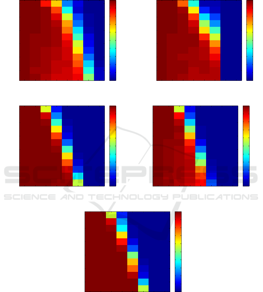
et al., 2011). Figure 2 depicts the empirical probabi-
lity of success 8 for OMP, CoSamp, AISS, GISS and
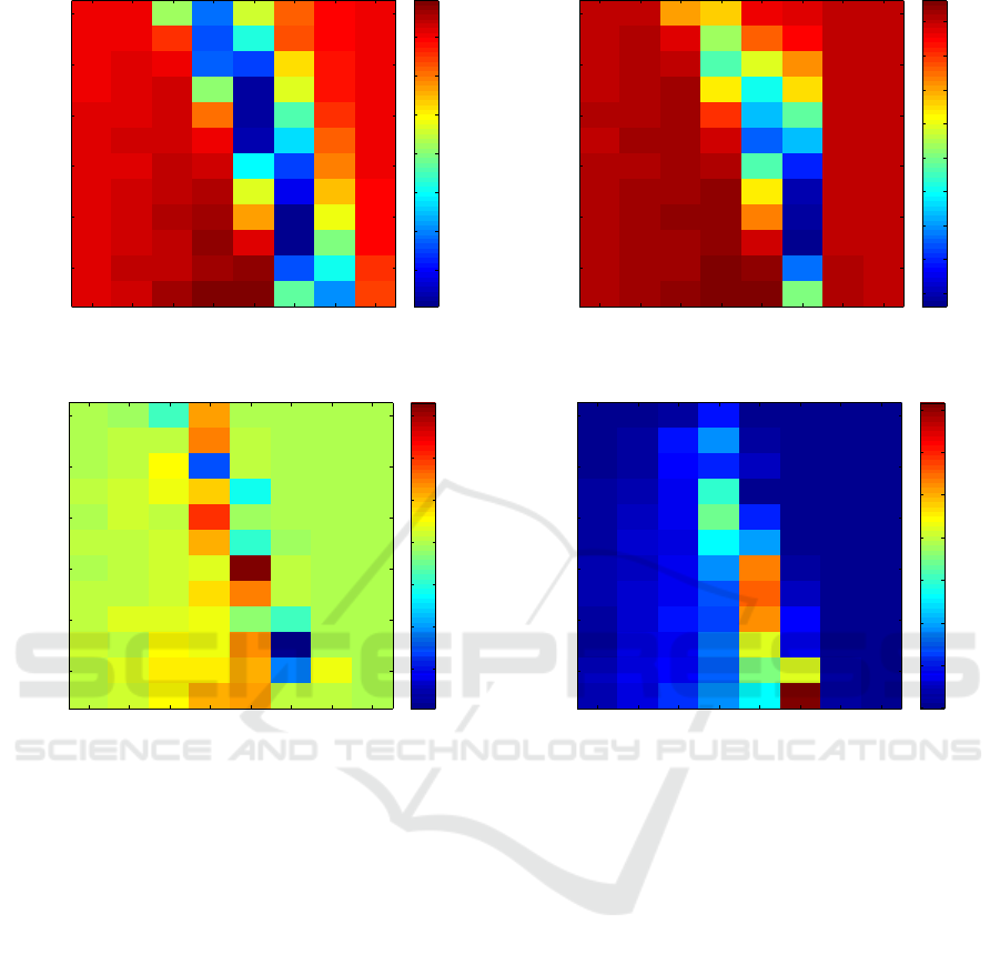
algorithm 1. We also consider the difference of pro-
bability of success between algorithm 1 and the other
methods:
D
pm,sq
:“ P
algo p1q
pm,sq
´ P
pm,sq
, (9)
where m P M, s P S, P
algo 1
pm,sq
(resp. P
pm,sq
) denotes the
quantity (8) obtained with algorithm 1 (resp. OMP,
CoSamp, AISS or GISS). It is easy to see that if (9)
is positive then algorithm 1 performed better than the
other method in terms of success as defined above.
These differences are depicted in figure 3. It is ea-
sily seen that OMP and CoSamp succeed at retrieving
the source signal with a probability of approximately
80% for a larger set of parameters than any other met-
hod. However, they produce correct results with a
probability of nearly 100% for a much smaller set of
parameters than AISS, GISS, and algorithm 1. An
overview of the similarities and differences between
OMP (Pati et al., 1993), CoSamp (Needell and Tropp,
2009), AISS (Burger et al., 2013) GISS (Moeller and
Zhang, 2016), and algorithm 1 is given in table 1. In
this table, we recall the assumption(s) on A, the va-
riables to maintain during the iterations, the update
rule and the type of convergence the method enjoys.
In table 1, we also give the empirical probability that
a least x% of signals are successfully reconstructed.
This statistical indicator is defined by
P
ěx
“
#
pm,sq P M ˆ S : P
pm,sq
ě x
(
#M ¨ #S
, (10)
A Simple and Exact Algorithm to Solve `
1
Linear Problems - Application to the Compressive Sensing Method
57
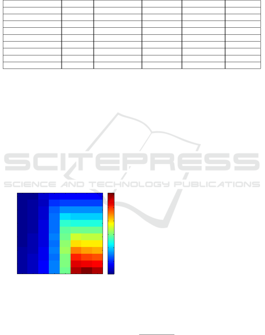
Table 1: Overview of main similarities and differences between OMP, CoSaMP, AISS, GISS and algorithm 1. Below,
ERC stands for exact recovery condition see, e.g., (Pati et al., 1993) and RIC stands for restricted isometry constant see,
e.g., (Needell and Tropp, 2009).
Method OMP (Pati et al., 1993) CoSamp (Needell and Tropp, 2009) AISS (Burger et al., 2013) GISS (Moeller and Zhang, 2016) Algorithm 1
Assumption(s) A satisfies ERC A satisfies RIC Du P R
n
: Au “ b A satisfies ERC A full row rank
Variable(s) u
k
P R
n
u
k
P R
n
u
k
P R
n
and p
k
P R
m
u
k
P R
n
and p
k
P R
m
λ
λ
λ
k
P R
m
Update(s) rule(s) least squares in R
n
least squares and hard threshold in R
n
constrained least squares in R
n
least squares in R
n
projection onto cone of R
m
Type of convergence Probabilistic Probabilistic Exact Exact Exact
Probability of at least 90 % of success (10) 0.5104 0.5521 0.4688 0.4063 0.4688
Probability of at least 95 % of success (10) 0.3854 0.4583 0.4375 0.3333 0.4479
Probability of at least 99 % of success (10) 0.1042 0.1250 0.3438 0.1042 0.4271
Probability of at least 99.9 % of success (10) 0 0 0.1250 0 0.3958
Probability of at least 100 % of success (10) 0 0 0.0521 0 0.3958
where P
pm,sq
is defined by (8). We now report results
concerning the number of iterations needed to achieve
convergence.
Figure 1 gives the average number of iterations
needed by algorithm 1. The maximal average number
of iterations is bounded from above by 600. Com-
paring figures 1 and 2 it can be noticed that when
the algorithm succeeds in recovering the source ele-
ment the average number of iterations remains below
(about) 250. This suggests modifying algorithm 1 to
use an early stopping criterion. The stopping criterion
would be either the optimality condition is reached or
a maximal number of iteration is attained. The com-
putational efficiency of the other algorithms conside-
red here can be found in, e.g., (Moeller and Zhang,
2016).
Pseudo l0 norm in percent
Number of observations
Average number of iterations
0.05 0.1 0.15 0.2 0.25 0.3 0.35 0.4
50
100
150
200
250
300
100
200
300
400
500
600
Figure 1: Average number of iteration needed by algo-
rithm 1. This figure suggest an early stopping criterion. See
text.
4 CONCLUSIONS
In this paper, a new fast algorithm to solve `
1
-
regularized linear problems was proposed. The algo-
rithm is exact: it produces an exact `
1
minimizer un-
der the constraints Au “ b in finite time. The method
relies on the calculation of a finite sequence of fea-
sible points of the dual. This sequence converges to
a solution of the dual problem. A solution of the pri-
mal problem is then obtained by a simple least squares
with signs constraints. Numerical comparisons with
existing methods of the literature has been proposed
for the noiseless compressive sensing (also called ba-
sis pursuit) problem. These comparisons allowed us
to illustrate the accuracy of the algorithm developed
in this paper compared to existing methods for the
compressive sensing paradigm. Indeed, the number
of parameters
2
where the `
1
reconstruction was nearly
always equal to the `
0
(sparsest) one is bigger with our
algorithm. The algorithm developed in this paper only
requires that A is full row rank. Hence, it can be used
in many problems. For instance, it can be applied with
matrices that do not comply with RIP-like properties.
The initialization of our algorithm was chosen arbitra-
rily as the null vector. Future work could investigate
the benefits of a smarter initial guess to further speed
up the method. Another ongoing work studies plausi-
ble stopping criteria.
ACKNOWLEDGEMENTS
The authors thanks Said Ladjal and Karim Trabelsi
for their fruitful comments. The authors also thank
the university of Valencia for its hospitality. The Aut-
hors thank M. Mller for providing the implementation
of the GISS algorithm.
2
`
0
pseudo norm, ambient dimension and dimension of
the observed data.
VISAPP 2018 - International Conference on Computer Vision Theory and Applications
58
Pseudo l0 norm in percent
Number of observations
Empirical probability of success: OMP
0.05 0.1 0.15 0.2 0.25 0.3 0.35 0.4
50
100
150
200
250
300
0.1
0.2
0.3
0.4
0.5
0.6
0.7
0.8
0.9
(a)
Pseudo l0 norm in percent
Number of observations
Empirical probability of success: CoSamp
0.05 0.1 0.15 0.2 0.25 0.3 0.35 0.4
50
100
150
200
250
300
0.1
0.2
0.3
0.4
0.5
0.6
0.7
0.8
0.9
(b)
Pseudo l0 norm in percent
Number of observations
Empirical probability of success: AISS
0.05 0.1 0.15 0.2 0.25 0.3 0.35 0.4
50
100
150
200
250
300
0
0.1
0.2
0.3
0.4
0.5
0.6
0.7
0.8
0.9
1
(c)
Pseudo l0 norm in percent
Number of observations
Empirical probability of success: GISS
0.05 0.1 0.15 0.2 0.25 0.3 0.35 0.4
50
100
150
200
250
300
0.1
0.2
0.3
0.4
0.5
0.6
0.7
0.8
0.9
(d)
Pseudo l0 norm in percent
Number of observations
Empirical probability of success: Algo1
0.05 0.1 0.15 0.2 0.25 0.3 0.35 0.4
50
100
150
200
250
300
0
0.1
0.2
0.3
0.4
0.5
0.6
0.7
0.8
0.9
1
(e)
Figure 2: Empirical probability of success (8). Panel (a): OMP (Pati et al., 1993), panel (b): CoSamp (Needell and Tropp,
2009), panel (c): AISS (Burger et al., 2013), panel (d) GISS (Moeller and Zhang, 2016) and panel (e) algorithm 1. The
non-zero entries of the source element u are drawn from a uniform distribution on r´1, 1s. The entries in A are drawn from
i.i.d. realization of a Gaussian distribution.
A Simple and Exact Algorithm to Solve `
1
Linear Problems - Application to the Compressive Sensing Method
59
Pseudo l0 norm in percent
Number of observations
Difference of empirical probability of success: OMP v.s. Algo1 tresh :1e−10
0.05 0.1 0.15 0.2 0.25 0.3 0.35 0.4
50
100
150
200
250
300
−0.6
−0.5
−0.4
−0.3
−0.2
−0.1
0
(a)
Pseudo l0 norm in percent
Number of observations
Difference of empirical probability of success: CoSamp v.s. Algo1 tresh :1e−10
0.05 0.1 0.15 0.2 0.25 0.3 0.35 0.4
50
100
150
200
250
300
−0.8
−0.7
−0.6
−0.5
−0.4
−0.3
−0.2
−0.1
0
(b)
Pseudo l0 norm in percent
Number of observations
Difference of empirical probability of success: AISS v.s. Algo1 tresh :1e−10
0.05 0.1 0.15 0.2 0.25 0.3 0.35 0.4
50
100
150
200
250
300
−0.06
−0.04
−0.02
0
0.02
0.04
0.06
(c)
Pseudo l0 norm in percent
Number of observations
Difference of empirical probability of success: GISS v.s. Algo1 tresh :1e−10
0.05 0.1 0.15 0.2 0.25 0.3 0.35 0.4
50
100
150
200
250
300
0
0.05
0.1
0.15
0.2
0.25
0.3
0.35
(d)
Figure 3: Difference of probability of success (9). Panel (a): Algo 1-OMP (Pati et al., 1993), panel (b): Algo 1-CoSamp (Nee-
dell and Tropp, 2009), panel (c): Algo 1-AISS (Burger et al., 2013) and panel (d) Algo 1-GISS (Moeller and Zhang, 2016).
A positive value indicates that algorithm 1 performs better, a negative value the contrary.
REFERENCES
Aubin, J.-P. and Cellina, A. (2012). Differential Inclusions:
Set-Valued Maps and Viability Theory. Grundlehren
der mathematischen Wissenschaften. Springer Berlin
Heidelberg.
Beck, A. and Teboulle, M. (2009). A fast iterative
shrinkage-thresholding algorithm for linear inverse
problems. SIAM Journal on Imaging Sciences,
2(1):183–202.
Blumensath, T. and Davies, M. E. (2009). Iterative hard
thresholding for compressed sensing. Applied and
Computational Harmonic Analysis, 27(3):265–274.
Br
´
ezis, H. (1973). Op
´
erateurs Maximaux Monotones et
Semi-Groupes de Contractions Dans Les Espaces de
Hilbert. North-Holland Publishing Co., American El-
sevier Publishing Co.
Burger, M., M
¨
oller, M., Benning, M., and Osher, S.
(2013). An adaptive inverse scale space method for
compressed sensing. Mathematics of Computation,
82(281):269–299.
Cand
`
es, E. J., Romberg, J., and Tao, T. (2006). Robust un-
certainty principles: Exact signal reconstruction from
highly incomplete frequency information. IEEE Tran-
sactions on information theory, 52(2):489–509.
Candes, E. J. and Tao, T. (2005). Decoding by linear pro-
gramming. Information Theory, IEEE Transactions
on, 51(12):4203–4215.
Candes, E. J. and Tao, T. (2006). Near-optimal signal re-
covery from random projections: Universal encoding
strategies? Information Theory, IEEE Transactions
on, 52(12):5406–5425.
Chen, S. S., Donoho, D. L., and Saunders, M. A. (2001).
Atomic decomposition by basis pursuit. SIAM review,
43(1):129–159.
Dai, W. and Milenkovic, O. (2009). Subspace pursuit for
compressive sensing signal reconstruction. Informa-
tion Theory, IEEE Transactions on, 55(5):2230–2249.
VISAPP 2018 - International Conference on Computer Vision Theory and Applications
60

Donoho, D. L. (2006). Compressed sensing. Information
Theory, IEEE Transactions on, 52(4):1289–1306.
Donoho, D. L. and Elad, M. (2003). Optimally sparse repre-
sentation in general (nonorthogonal) dictionaries via
`1 minimization. Proceedings of the National Aca-
demy of Sciences, 100(5):2197–2202.
Foucart, S. (2013). Stability and robustness of weak ort-
hogonal matching pursuits. In Recent advances in
harmonic analysis and applications, pages 395–405.
Springer.
Grant, M. C. and Boyd, S. P. The CVX Users Guide, Release
2.1.
Hale, E. T., Yin, W., and Zhang, Y. (2007). A Fixed-
Point Continuation Method for l1-Regularized Mini-
mization with Applications to Compressed Sensing.
CAAM Technical Report TR07-07.
Hiriart-Urruty, J.-B. and Lemarechal, C. (1996a). Convex
Analysis and Minimization Algorithms I: Fundamen-
tals. Grundlehren der mathematischen Wissenschaf-
ten. Springer Berlin Heidelberg.
Hiriart-Urruty, J.-B. and Lemarechal, C. (1996b). Convex
Analysis and Minimization Algorithms II: Advanced
Theory and Bundle Methods. Grundlehren der mat-
hematischen Wissenschaften. Springer Berlin Heidel-
berg.
Jain, P., Tewari, A., and Dhillon, I. S. (2011). Orthogonal
matching pursuit with replacement. In Advances in
Neural Information Processing Systems, pages 1215–
1223.
Maleki, A. (2009). Coherence analysis of iterative thres-
holding algorithms. In Communication, Control, and
Computing, 2009. Allerton 2009. 47th Annual Aller-
ton Conference on, pages 236–243. IEEE.
Maleki, A. and Donoho, D. L. (2010). Optimally tuned ite-
rative reconstruction algorithms for compressed sen-
sing. IEEE Journal of Selected Topics in Signal Pro-
cessing, 4(2):330–341.
Mallat, S. and Zhang, Z. (1993). Matching pursuits with
time-frequency dictionaries. Signal Processing, IEEE
Transactions on, 41(12):3397–3415.
Meyer, M. C. (2013). A simple new algorithm for quadratic
programming with applications in statistics. Commu-
nications in Statistics-Simulation and Computation,
42(5):1126–1139.
Moeller, M. and Zhang, X. (2016). Fast Sparse Recon-
struction: Greedy Inverse Scale Space Flows. Mat-
hematics of Computation, 85(297):179–208.
Needell, D. and Tropp, J. A. (2009). CoSaMP: Iterative
signal recovery from incomplete and inaccurate sam-
ples. Applied and Computational Harmonic Analysis,
26(3):301–321.
Needell, D. and Vershynin, R. (2009). Uniform uncertainty
principle and signal recovery via regularized orthogo-
nal matching pursuit. Foundations of computational
mathematics, 9(3):317–334.
Osher, S., Burger, M., Goldfarb, D., Xu, J., and Yin, W.
(2005). An iterative regularization method for to-
tal variation-based image restoration. Multiscale Mo-
deling & Simulation, 4(2):460–489.
Pati, Y. C., Rezaiifar, R., and Krishnaprasad, P. (1993). Ort-
hogonal matching pursuit: Recursive function approx-
imation with applications to wavelet decomposition.
In Conference Record of The Twenty-Seventh Asilo-
mar Conference on Signals, Systems and Computers,
pages 40–44. IEEE.
Rockafellar, R. T. (1997). Convex Analysis. Princeton Uni-
versity Press, Princeton, NJ.
Tropp, J. A. and Gilbert, A. C. (2007). Signal recovery
from random measurements via orthogonal matching
pursuit. Information Theory, IEEE Transactions on,
53(12):4655–4666.
Yin, W., Osher, S., Goldfarb, D., and Darbon, J. (2008).
Bregman iterative algorithms for zell 1-minimization
with applications to compressed sensing. SIAM Jour-
nal on Imaging Sciences, 1(1):143–168.
Zhang, X., Burger, M., and Osher, S. (2011). A unified
primal-dual algorithm framework based on bregman
iteration. Journal of Scientific Computing, 46(1):20–
46.
APPENDIX
Program Code
Matlab code for algorithm 1.
function [solution_primal,solution_dual,nb_iteration]=compute_solution_l1(A,
...,observed_vect, param)
% Step. 0 Initialization
lambda_init=param.initdual;
A=[A -A];
%% Step1. Compute solution dual
[solution_dual,active_set,nb_iteration]=compute_solution_dual(A,
observed_vect,...,lambda_init,param);
%% Step2. Compute solution primal
solution_primal=compute_solution_primal(A,observed_vect,active_set,param);
%%%%%%%%%%%%%%%%%%%%%%%%%%%%%%%%%%%%%%%%%%%%%%%%%%%%%%%%%%%%%%%%%%%%%%%%%
%%%%%%%%%%%%%%%%%%%%%%%%%%%%%%%%%%%%%%%%%%%%%%%%%%%%%%%%%%%%%%%%%%%%%%%%%
%%%%%%%%%%%%%NESTED FUNCTIONS: Compute Dual + Primal %%%%%%%%%%%%%%%%%%%%
%%%%%%%%%%%%%%%%%%%%%%%%%%%%%%%%%%%%%%%%%%%%%%%%%%%%%%%%%%%%%%%%%%%%%%%%%
%%%%%%%%%%%%%%%%%%%%%%%%%%%%%%%%%%%%%%%%%%%%%%%%%%%%%%%%%%%%%%%%%%%%%%%%%
%%%%%%%%%%%%%%%%%%%%%%%%%%%%%%%%%%%%%%%%%%%%%%%%%%%%%%%%%%%%%%%%%%%%%%%%%
%%%%%%%%%%%%%%%%%%%%%%%%%% Compute_solution_dual %%%%%%%%%%%%%%%%%%%%%%%
%%%%%%%%%%%%%%%%%%%%%%%%%%%%%%%%%%%%%%%%%%%%%%%%%%%%%%%%%%%%%%%%%%%%%%%%%
function [lambda,active_set,nb_iteration]=compute_solution_dual(A,
observed_vect,...,lambda,param)
%% 0. Initialize DO WHILE loop and pre-compute some stuff
shall_continue=true;
Atransp=A’;
nb_iteration=0;
while shall_continue
% 1. Compute active set
active_set=compute_active_set(A,lambda,param);
% 2. Compute direction
direction=compute_direction(A,observed_vect,active_set,param);
% 3. Compute kick time
timestep=compute_kick_time(A,direction,lambda,param);
% 4. Check termination condition
if (norm(direction*timestep)<param.tolcomputedual...
||norm(direction)<param.tolcomputedual||timestep==realmax)
% 5.1 Stop
shall_continue=false;
else % 5.2 Move current point in dual
A Simple and Exact Algorithm to Solve `
1
Linear Problems - Application to the Compressive Sensing Method
61

lambda=update_lambda(Atransp,lambda,direction,timestep,param);
end; % endif
nb_iteration=nb_iteration+1
end; % end whil
end % end compute_solution_dual function
%%%%%%%%%%%%%%%%%%%%%%%%%%%%%%%%%%%%%%%%%%%%%%%%%%%%%%%%%%%%%%%%%%%%%%%%%
%%%%%%%%%%%%%%%%%%%%%%%%%%%%%%%%%%%%%%%%%%%%%%%%%%%%%%%%%%%%%%%%%%%%%%%%%
%%%%%%%%%%%%%%%%%%%%%%%%%%%%%%%%%%%%%%%%%%%%%%%%%%%%%%%%%%%%%%%%%%%%%%%%%
%%%%%%%%%%%%%%%%%%%%%%%%%% update_lambda %%%%%%%%%%%%%%%%%%%%%%%%%%%%%%%%
%%%%%%%%%%%%%%%%%%%%%%%%%%%%%%%%%%%%%%%%%%%%%%%%%%%%%%%%%%%%%%%%%%%%%%%%%
function lambda=update_lambda(Atransp,lambda,direction,...
timestep,param)
% 0. Safery check : if not valid set t to 0 then quit (termination valid)
if isempty(timestep) timestep=0; end; %end if
% 1. Move in dual feasible set
lambda=lambda+timestep*direction;
% 1.1 : reproject new positon onto feasible set
if (param.leastquarefit_flag)
% compute projection onto dual feasible set
norm_Atransplambda=max(abs(Atransp*lambda))+param.tolcomputedual;
if (norm_Atransplambda>1+param.tolcomputedual)
lambda=(1+param.tolcomputedual)*lambda/norm_Atransplambda;
end;
end; % end if
end % end: update_lambda functon
%%%%%%%%%%%%%%%%%%%%%%%%%%%%%%%%%%%%%%%%%%%%%%%%%%%%%%%%%%%%%%%%%%%%%%%%%
%%%%%%%%%%%%%%%%%%%%%%%%%%%%%%%%%%%%%%%%%%%%%%%%%%%%%%%%%%%%%%%%%%%%%%%%%
%%%%%%%%%%%%%%%%%%%%%%%%%%%%%%%%%%%%%%%%%%%%%%%%%%%%%%%%%%%%%%%%%%%%%%%%%
%%%%%%%%%%%%%%%%%%%%%%%%%% compute_active_set %%%%%%%%%%%%%%%%%%%%%%%%%%%
%%%%%%%%%%%%%%%%%%%%%%%%%%%%%%%%%%%%%%%%%%%%%%%%%%%%%%%%%%%%%%%%%%%%%%%%%
function active_set=compute_active_set(A,lambda,param)
active_set=(((lambda’)*A)>=1-param.tolcomputedual);
end % end : compute_active_set function
%%%%%%%%%%%%%%%%%%%%%%%%%%%%%%%%%%%%%%%%%%%%%%%%%%%%%%%%%%%%%%%%%%%%%%%%%
%%%%%%%%%%%%%%%%%%%%%%%%%%%%%%%%%%%%%%%%%%%%%%%%%%%%%%%%%%%%%%%%%%%%%%%%%
%%%%%%%%%%%%%%%%%%%%%%%%%%%%%%%%%%%%%%%%%%%%%%%%%%%%%%%%%%%%%%%%%%%%%%%%%
%%%%%%%%%%%%%%%%%%%%%%%%%% compute_direction %%%%%%%%%%%%%%%%%%%%%%%%%%%%
%%%%%%%%%%%%%%%%%%%%%%%%%%%%%%%%%%%%%%%%%%%%%%%%%%%%%%%%%%%%%%%%%%%%%%%%%
function direction=compute_direction(A,observed_vect,active_set,param)
% the next is equal to the proj of 0 onto the set b+ active cols of A
direction=-observed_vect-projection_simplicial_cone(A,-observed_vect,...
active_set,param);
end % end : compute_direction function
%%%%%%%%%%%%%%%%%%%%%%%%%%%%%%%%%%%%%%%%%%%%%%%%%%%%%%%%%%%%%%%%%%%%%%%%%
%%%%%%%%%%%%%%%%%%%%%%%%%%%%%%%%%%%%%%%%%%%%%%%%%%%%%%%%%%%%%%%%%%%%%%%%%
%%%%%%%%%%%%%%%%%%%%%%%%%%%%%%%%%%%%%%%%%%%%%%%%%%%%%%%%%%%%%%%%%%%%%%%%%
%%%%%%%%%%%%%%%%%%%%%%%%%% compute_kick_time %%%%%%%%%%%%%%%%%%%%%%%%%%%%
%%%%%%%%%%%%%%%%%%%%%%%%%%%%%%%%%%%%%%%%%%%%%%%%%%%%%%%%%%%%%%%%%%%%%%%%%
function t=compute_kick_time(A,direction,lambda,param)
% 0. Compute S_Cˆ+(lambda) set
active_set_plus=(((direction’)*A)>param.tolcomputedual);
% 1. Compute kick time
% 1.1: verify possible emptyness
if (˜any(active_set_plus)) % empty active set
t=realmax; %’+infty (from its definition)
else
% 1.2 non empty case
Aactiveplus=A(:,active_set_plus);
t=min((1-((lambda’)*Aactiveplus))./((direction’)*Aactiveplus));
% safety check t must be non negative
if (t<0) t=0; % we set t:=0; then quit (termination condition valid)
end;
end; % end if
end % end: compute_kick_time function
%%%%%%%%%%%%%%%%%%%%%%%%%%%%%%%%%%%%%%%%%%%%%%%%%%%%%%%%%%%%%%%%%%%%%%%%%
%%%%%%%%%%%%%%%%%%%%%%%%%% compute_solution_primal %%%%%%%%%%%%%%%%%%%%%%
%%%%%%%%%%%%%%%%%%%%%%%%%%%%%%%%%%%%%%%%%%%%%%%%%%%%%%%%%%%%%%%%%%%%%%%%%
function sol_primal=compute_solution_primal(A,observed_vect,...
active_set,param)
[˜,sol_primal]=projection_simplical_cone(A,-observed_vect,...
active_set,param);
sol_primal=-sol_primal(1:end/2)+sol_primal(end/2+1:end);
end % end : compute_solution_primal function
%%%%%%%%%%%%%%%%%%%%%%%%%%%%%%%%%%%%%%%%%%%%%%%%%%%%%%%%%%%%%%%%%%%%%%%%%
%%%%%%%%%%%%%%%%%%%%%%%%%%%%%%%%%%%%%%%%%%%%%%%%%%%%%%%%%%%%%%%%%%%%%%%%%
%%%%%%%%%%%%%%%%%%%%%%%%%%%%%%%%%%%%%%%%%%%%%%%%%%%%%%%%%%%%%%%%%%%%%%%%%
%%%%%%%%%%%%%%%%%%%%%%%%%%%%%%%%%%%%%%%%%%%%%%%%%%%%%%%%%%%%%%%%%%%%%%%%%
%%%%%%%%%%%%%%%%%%%%%%%%%%%%%%%%%%%%%%%%%%%%%%%%%%%%%%%%%%%%%%%%%%%%%%%%%
%%%%%%%%%%%%%%%%%%%%%%%%%%%%%%%%%%%%%%%%%%%%%%%%%%%%%%%%%%%%%%%%%%%%%%%%%
%%%%%%%%%%%%%%%%%%%%%%%%%%%%%% END NESTED FUNCTIONS%%%%%%%%%%%%%%%%%%%%%%
%%%%%%%%%%%%%%%%%%%%%%%%%%%%%%%%%%%%%%%%%%%%%%%%%%%%%%%%%%%%%%%%%%%%%%%%%
%%%%%%%%%%%%%%%%%%%%%%%%%%%%%%%%%%%%%%%%%%%%%%%%%%%%%%%%%%%%%%%%%%%%%%%%%
end% end: compute_solution_l1 function
Notations
(i) (Vectors) Vectors of, e.g., R
n
are denoted in
bold typeface, e.g., x. Other objects like scalars
or functions are denoted in non-bold typeface
(ii) (Inner product) xx, yy “
ř
i
x
i
y
i
(iii) (the `
8
pR
n
q unit ball) B
8
“
tu : xu,e
i
y ď 1, i “ 1, .. ., 2nu where e
i
de-
notes the canonical vector
(iv) (Effective domain) dom f : The domain of a
convex function f is the (convex, possibly
empty) set dom f “ tx P R
n
: f pxq P Ru
(v) (Convex function) A function f : R
n
Ñ R Y
t`8u is said to be convex if @px, yq P R
n
ˆ R
n
and @α P p0, 1q f pαx ` p1 ´ αqyq ď α f pxq `
p1 ´ αq f pyq holds true (in R Y t`8u)
(vi) (Set Γ
0
pR
n
q) The set of lower semi-continuous,
convex functions with dom f ‰ H is denoted
by Γ
0
pR
n
q
(vii) (Characteristic function of a set) χ
E
pxq “ 0 if
x P E and χ
E
pxq “ `8 otherwise
(viii) (Right derivative)
d
`
λ
λ
λptq
dt
:“
lim
hÑ0
`
λ
λ
λpt`hq´λ
λ
λptq
h
(ix) (Convex conjugate) For any f convex that sa-
tisfies dom f ‰ H, the function f
˚
defined by
R
n
Q s ÞÑ f
˚
psq :“ sup
xPdom f
txs,xy´ f pxqu.
(See , e.g., (Hiriart-Urruty and Lemarechal,
1996b, Def. 1.1.1, p. 37))
(x) (Euclidean projection) Π
C
pxq “ arg min
yPC
}y´
x}
`
2
for C ‰ H closed and convex
VISAPP 2018 - International Conference on Computer Vision Theory and Applications
62
