A Hybrid CPU-GPU Scalable Strategy for Multi-resolution Rendering of

Large Digital Elevation Models with Borders and Holes

Andrey Rodrigues and Waldemar Celes

Tecgraf/PUC-Rio Institute, Computer Science Department,

Pontiﬁcal Catholic University of Rio de Janeiro, Rio de Janeiro, Brazil

Keywords:

Digital Elevation Model, Terrain Rendering, Scalable LOD, GPU Tessellation.

Abstract:

Efﬁcient rendering of large digital elevation models remains as a challenge for real-time applications, espe-

cially if those models contain irregular borders and holes. First, direct use of hardware tessellation has limited

scalability; although the graphics hardware is capable of controlling the resolution of patches in a very efﬁ-

cient manner, the whole patch data must be loaded in memory. Second, previous techniques restrict elevation

data resolution and do not handle irregular border or holes. In this paper, we propose an efﬁcient and scalable

hybrid CPU-GPU algorithm for rendering large digital elevation models. Our proposal effectively combines

GPU tessellation with CPU tile management, taking full advantage of GPU processing capabilities while main-

taining graphics-memory use under practical limits. Our proposal also handles models with irregular borders

and holes. Additionally, we present a technique to manage level of detail of aerial imagery mapped on top

of elevation models. Both geometry and texture level of detail management run independently, and tiles are

combined with no need to load extra data.

1 INTRODUCTION

Due to advances in acquisition technologies, large

digital elevation models (DEM), with gigabytes of

data, have been widely available. As a consequence,

an efﬁcient and scalable rendering technique for such

models has been mandatory in different applications.

Without any special treatment, the amount of data eas-

ily exceeds hardware limits in both memory and tri-

angle throughput.

On the other hand, graphics hardware tessellation

has evolved and is currently able to generate complex

geometry on the ﬂy (Schäfer et al., 2014), eliminat-

ing the need to generate the geometry on the CPU,

and thus avoiding transferring a large amount of data

to the graphics pipeline at each frame. In this paper,

we present a hybrid CPU-GPU strategy for handling

large elevation models. Previous works have also

taken advantage of hardware tessellation for DEM

rendering (Yusov and Shevtsov, 2011; Fernandes and

Oliveira, 2012; Kang et al., 2015), trying different

strategies for mapping CPU tiles to GPU patches and

for avoiding cracks along patch interfaces. Our hy-

brid approach makes it possible to control both CPU

and GPU memory and computational loads, by tuning

CPU-tile and GPU-patch sizes, and avoids cracks by

construction.

Furthermore, previous proposals on rendering dig-

ital elevation models restrict tile/patch resolutions,

generally as (2

+ 1)× (2

+ 1), and do not handle ir-

regular borders and holes. We present a new method

for handling borders and holes in DEMs. We intro-

duce a metric to compute horizontal errors due to bor-

der displacements, as tile/patch resolution is reduced,

and ensure these errors are under control in our level-

of-detail management. Our approach also imposes re-

strictions on tile/patch resolution; however, being able

to deal with holes allows us to easily handle models in

arbitrary resolutions by just ﬁlling the “blanks” with

holes. As we shall demonstrate, we are then able to

render very long terrain strips and large seismic sur-

faces with complex holes.

We then extend our proposal to also manage level

of detail of aerial imagery mapped as textures on top

of elevation models. The texture tiles are also stored

in a quadtree structure and the active cut is mandated

by the screen resolution of projected tiles. Both ge-

ometry and texture level-of-detail managements run

independently. As a result, we may end up with a 1-

to-n or n-to-1 mapping between geometry and texture

tiles; both cases are handled smoothly without any ad-

ditional load of data.

The rest of this paper is organized as follows. In

the next section, we discuss related work. Then we

240

Rodrigues, A. and Celes, W.

A Hybrid CPU-GPU Scalable Strategy for Multi-resolution Rendering of Large Digital Elevation Models with Borders and Holes.

DOI: 10.5220/0006621902400247

In Proceedings of the 13th International Joint Conference on Computer Vision, Imaging and Computer Graphics Theory and Applications (VISIGRAPP 2018) - Volume 1: GRAPP, pages

240-247

ISBN: 978-989-758-287-5

present our strategy, discuss how we handle irregu-

lar borders and holes, and describe how we combine

aerial level of detail. Next, we present the results of

several computational experiments. Finally, we draw

concluding remarks.

2 RELATED WORK

Several researches have been done to efﬁciently ren-

der massive terrain data. In (Pajarola and Gobbetti,

2007), the authors presented a comprehensive survey

on multi-resolution approaches for digital terrain ren-

dering, analyzing different choices of data structures

and error metrics. The general idea consists in struc-

turing the data in an hierarchical way to manage adap-

tive level of detail.

Early multi-resolution approaches have opted for

a triangle-based hierarchy. Binary tree hierarchies

were proposed to control triangulation resolution

based on a screen-space error evaluation (Lindstrom

et al., 1996) (Duchaineau et al., 1997) (Lindstrom and

Pascucci, 2001). While simple to implement, these

techniques are limited by CPU-GPU memory transfer

because the geometry has to be loaded to the GPU for

every frame.

In order to overcome this limitation, techniques

such as BDAM (Cignoni et al., 2003a) and P-BDAM

(Cignoni et al., 2003b) opted for a tile-based hier-

archy: each hierarchical node represents a precom-

puted triangle surface tile instead of a single trian-

gle. The elevation data, which is encoded using a

wavelet-based compression technique, can be placed

into the GPU memory for future use. The use of a

tile-based hierarchy is scalable and efﬁcient, at the

cost of decreased adaptivity, processing more trian-

gles than needed. Geometry clipmaps (Losasso and

Hoppe, 2004) use a mipmap pyramid as the terrain

representation and a compression technique to reduce

the storage requirements; however, they simpliﬁed the

evaluation of the screen-space error to choose the ap-

propriate level of detail, thus affecting resulting image

quality.

Recent approaches have tried to explore the GPU

tessellation to speedup mesh generation. A crack-free

terrain surface generation with a continuous LOD tri-

angulation algorithm is presented in (Fernandes and

Oliveira, 2012). The method simply estimates the size

of a patch in screen-space and tessellates it accord-

ingly, producing a constant triangle size in pixels. In

(Cervin, 2012), a density map is used, which encodes

the terrain curvature, to choose the appropriate level

of detail in the GPU tessellation stage, creating more

triangles for a high density area (bumpy land) and few

triangles for low density areas (ﬂat land). However,

these techniques do not accurately evaluate geometry

errors in the ﬁnal triangulation.

The approach proposed in (Yusov and Shevtsov,

2011) is similar to ours. They also subdivide the

model in patches (we call tiles) and then in blocks (we

call patches). However, their approach is not able to

ensure, by construction, crack-free surface along tile

interfaces. To hide gaps along tile interface, they ex-

ploit “vertical skirts” as proposed in (Ulrich, 2000).

Also, no analysis is performed to justify the choice

of tile and patch resolutions. On another hand, Kang

et al. (Kang et al., 2015) have presented an strategy

for avoiding cracks by construction, annotating four

edge LODs for each quadtree node (tile), determined

by using the inner LODs of the current node and its

neighbors. As in their approach each tile is mapped to

a single patch, all tessellation levels are computed in

CPU. We use a similar strategy to avoid crack along

tile interfaces, but our approach maps each CPU tile

to a set of GPU patches, minimizing CPU load. As

a consequence, we also need to avoid cracks along

patch interfaces.

3 GEOMETRY LOD

The proposed algorithm to render multi-resolution el-

evation models is a hybrid CPU-GPU approach. The

CPU is responsible for managing a quadtree of tiles.

Each tile is subdivided into a set of patches that are

sent to the GPU, as illustrated in Figure 1.

3.1 Pre-processing Phase

In a pre-processing phase, the quadtree is built ap-

plying a bottom-up procedure. First, the tile resolu-

tion is chosen, and different choices of resolution af-

fect memory footprint and performance, as we shall

see. The whole elevation data is subdivided into tiles

representing the quadtree leafs. Then, for each four

neighbors, a parent tile is created with half of the chil-

dren’s resolution, ﬁlling the quadtree top levels. For

simplicity, we do not apply any ﬁlter for reducing tile

resolution; we only eliminate each other line/column

of data, avoiding discontinuities along tile interfaces.

The resolution of each patch, and consequently

the number of patches per tile, also affects perfor-

mance. The maximum resolution is limited by the

graphics hardware. In Section 6, we present the com-

putational test we ran to test different resolutions.

Once tile and patch resolutions are chosen, we are

ready to compute the errors in object space associated

to each tile and each patch.

A Hybrid CPU-GPU Scalable Strategy for Multi-resolution Rendering of Large Digital Elevation Models with Borders and Holes

241

n x n

patches

Figure 1: Geometry tiles are selected to honor a predeﬁned

screen-space error limit; each tile is subdivided into a ﬁxed

number of patches to the GPU.

Tile and patch resolutions must be of dimension

+1)× (2

+1), because neighbor tiles (or patches)

share the same border pixels. For simplicity, we men-

tion dimension values by power of two (2

× 2

To illustrate the discussion that follows, let us con-

sider that tile’s resolution is 512 × 512 and patch’s is

64× 64. So, each tile is subdivided into 8× 8 patches.

For each tile, we ﬁrst compute the error in ob-

ject space associated to each patch for different res-

olutions. For the leaf tiles, the error for each patch

at maximum resolution is zero. We denote this by

= 0, where i represents the patch, l the tile

quadtree level, and 64 the patch tessellation level. For

each patch, we then annotate the errors associated to

smaller tessellation levels: ε

, ε

, · · · , ε

The error in object space associated to a tile is

given by: E

= max

, being naturally zero for the

leaf tiles. The errors of patches at upper quadtree lev-

els are inherited from the lower levels with half of the

maximum tessellation:

l−1

= max

i∈N

(1)

where N represents the set of associated four neigh-

boring patches. This error is then propagated to

smaller tessellation levels and, again, the tile error is

l−1

= max

l−1

. For each tile, all patch errors are

annotated and stored in a texture to be accessed in

the GPU-tessellation stage. Figure 2 illustrates this

object-space error computation.

3.2 Rendering Phase

At run time, the error in screen space ρ is computed

in the usual way, either to select tiles on the CPU or

to determine patch tessellation level on the GPU:

ρ = λ

, with λ =

2tan

(2)

where E, w, θ and d represent, respectively, the er-

ror in object space, the viewport resolution, the cam-

era ﬁeld of view and the distance from the camera to

the closest point of the tile’s (or patch’s) 3D bounding

box.

Compute

11632

,...,







111

11632

3264

,...,

,max











Compute







1l

Figure 2: Computed object-space errors: at leaf tiles, for

each patch at maximum tessellation level, the associated er-

ror is zero; errors are then propagated to other possible tes-

sellation levels. Errors of patches at upper quadtree level

are inherited from the lower levels. The error associated to

each tile is the maximum annotated to patches at maximum

tessellation level.

On the CPU, we use two threads to process the

data. The loading thread is responsible for predicting

camera movement and loading tiles in advance from

disk. The rendering thread is responsible for select-

ing tiles, among the loaded ones, necessary to render

the terrain honoring a prescribed error tolerance for

the current frame. Both threads use the conventional

top-down approach, subdividing the tile if the screen

space error exceed the prescribed tolerance.

Once the frame tiles are selected, the CPU is re-

sponsible for issuing rendering commands for the cor-

responding patches. In the tessellation shader, the

level of detail of each patch is determined. The inner

tessellation level is given by evaluating the screen-

space error of the patch, choosing the lowest pos-

sible resolution. The choice of the outer tessella-

tion level must avoid T-junctions between adjacent

patches. There are two cases, denoted here by the

patch-patch case, for interfaces between two patches

of a same tile, and the tile-tile case, for interfaces be-

tween patches of different tiles.

The patch-patch case is easily handled, because

all the needed data are available within the tile. The

outer tessellation level is given by the maximum sub-

division requested by the interfacing patches, as in

(Yusov and Shevtsov, 2011). So, the coarsest patch

gets reﬁned along the border:

outer

= max(n

) (3)

where n

and n

represents the computed inner level

of the interfacing patches.

The challenge lies on the tile-tile case; data are not

available within a tile and additional information is

necessary. To overcome this problem, on the CPU, af-

ter performing the LOD algorithm (tile selection), for

each tile, we annotate the difference in level between

GRAPP 2018 - International Conference on Computer Graphics Theory and Applications

242

adjacent selected tiles; one value for each tile edge.

If the level of the adjacent tile is equal or higher (the

adjacent is more reﬁned), we annotate the value zero;

if the level of the adjacent tile is lower (it is less re-

ﬁned), we annotate the difference in level: l

tile

− l

ad j

Figure 3 illustrates the values annotated for a sample

active quadtree. In the tessellation shader, the outer

tessellation level of a tile-tile interface is given by:

outer

max

(4)

where n

max

is the maximum possible subdivision for

the patch and δ is the annotated level difference. This

imposes a limit in the unbalance level of adjacent tiles

equals to log

max

, which, in practice, tends not to

be a problem. For instance, for a 64 × 64 patch res-

olution, the unbalance between adjacent tiles cannot

exceed a factor of six. If this limit is reached, it is im-

posed a subdivision on the less reﬁned tile. All patch

borders along the tile edge get the same outer tessel-

lation level. Note that this approach makes all inter-

face between tiles reﬁned to the most possible reso-

lution. This induces a small increase in the number

of generated triangles but makes it simple to avoid

T-junctions. As we shall demonstrate, this approach

to ensure crack-free surface does not impact perfor-

mance. Moreover, there is no need to employ ad-

ditional procedures for crack ﬁlling, such as to add

ﬂanges, to join tiles with special meshes, or to gener-

ate vertical ribbon meshes(Ulrich, 2000).

0 1

0 0

1 0 0

Figure 3: Annotated level differences along tile edges.

For each edge of a selected tile, the neighboring tiles are

checked; if neighbor tile is at same or higher level, zero is

annotated; if neighbor tile is at lower level, level difference

is annotated.

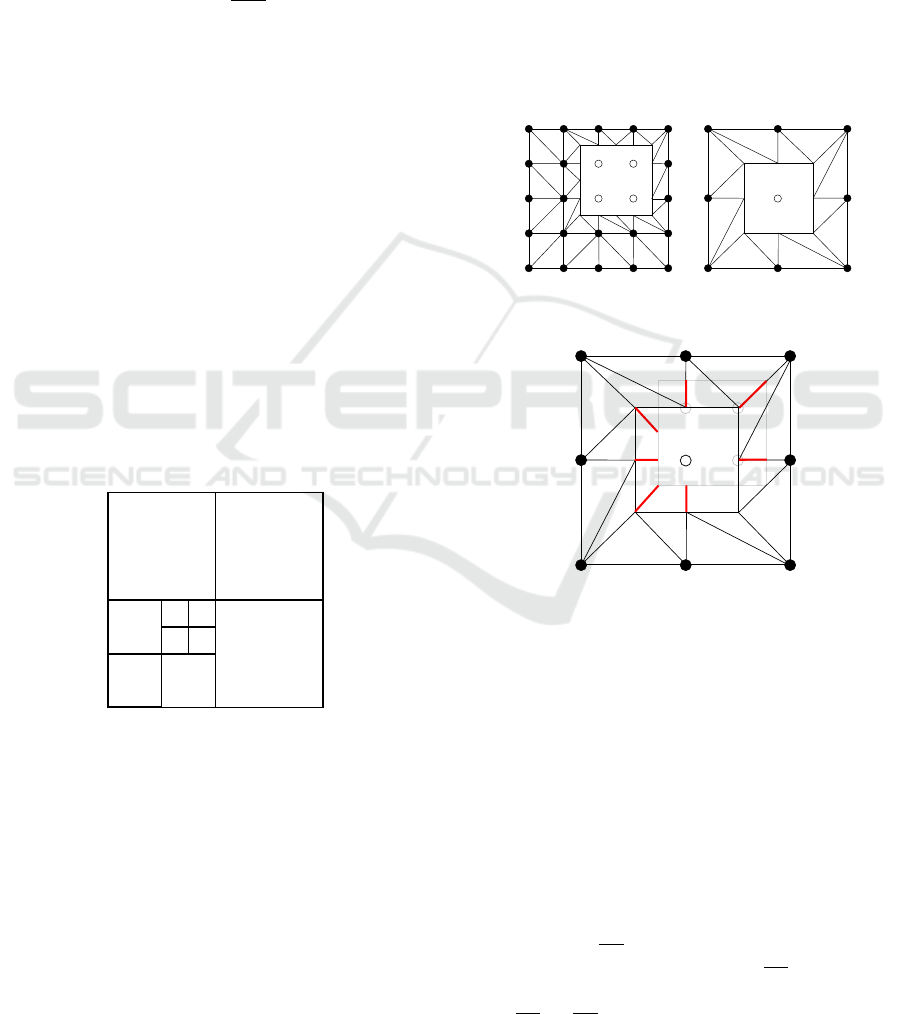
4 BORDERS AND HOLES

We now extend our approach to deal with irregular

borders and holes. In such models, there are regular

vertices (•) and void vertices (◦). We then consider

that there are borders along all the interfaces between

regular and void vertices. Figure 4a (left) illustrates

a 4 × 4 patch with four void vertices and the corre-

sponding deﬁned border. At ﬁrst, void vertices have

no associated elevation data. In order to render the

border, in a pre-processing phase, we assign, to each

void vertex, an elevation value given by its neighbor-

ing regular vertices.

For computing the error in object space when de-

creasing tile/patch resolution, we need to consider

border displacements, which we identify as horizon-

tal error. Figure 4 shows what happens when decreas-

ing the resolution of the illustrative patch from 4 × 4

to 2 × 2 (Figure 4a). As each other line/column are

eliminated, the border is displaced, and horizontal er-

ror, illustrated in Figure 4b, has to be considered.

(a)



(b)

Figure 4: Horizontal object space errors: (a) illustrative

patch with void vertices and corresponding coarser level;

(b) computed horizontal errors due to border displacement.

Table 1 summarizes all possible cases involving

void vertices when reducing resolution. For each

eliminated vertex in a patch, the error is computed

considering removing the middle vertex of four edges:

horizontal, vertical, forward diagonal, and backward

diagonal. The maximum error is stored per patch con-

sidering all edges of all eliminated vertices. Let as

take as example the second table entry, case A−C − B

as • − • − ◦ (regular, regular, and void vertices), where

vertex C is removed: originally, the border is in the

middle of edge

CB; after removing vertex C, the bor-

der is moved to the middle of edge AB, representing

a displacement equal to ∆/2, where ∆ is the length of

edge AC (or BC).

A Hybrid CPU-GPU Scalable Strategy for Multi-resolution Rendering of Large Digital Elevation Models with Borders and Holes

243

Vertical errors are expressed in the usual way by:



+ z

− z



(5)

where z

represents the elevation value at vertex V .

This is valid for all cases, except for the last table

entry, involving only void vertices; in this case, both

vertical and horizontal errors are zero.

In the pre-processing phase, both maximum errors

are annotated. The combined error, expressed by:

E =

+ E

(6)

is only computed in the rendering phase. The reason

we do that is to allow applying a vertical scale fac-

tor when visualizing the model, which is commonly

employed.

In the rendering phase, the combined error is pro-

jected to compute the error in screen space. Note that

the whole patch is rendered, even triangles with void

vertices. In order to correctly render the border, we

assign an attribute equal to one for regular vertices

and equal to zero for void vertices. This attribute

is interpolated by the rasterizer and, in the fragment

shader, fragments with attribute value less than 0.5

are discarded.

Patches with only void vertices are not rendered,

and tiles with only void vertices are not even rep-

resented in the quadtree. This allows us to pro-

cess rectangular elevation data using regular quadtree

in a effective way. The rectangular data is com-

pleted with void vertices to get the required resolu-

tion (2

+ 1 × 2

+ 1) but, in the end, we get a non-

complete quadtree, as void tiles are discarded.

5 TEXTURE LOD

On top of the multi-resolution elevation surface, we

map aerial imagery as textures, also managing its

Table 1: Table of corresponding horizontal (E

) errors when

eliminating a vertex C in the middle of an edge AB. The

value of ∆ corresponds to the horizontal length of AC or CB.

Note that the edge AB may be horizontal, vertical, forward

diagonal, or backward diagonal, with respect to the patch.

A − C − B E

• − • − • 0

• − • − ◦ ∆/2

• − ◦ − • ∆

• − ◦ − ◦ ∆/2

◦ − • − • ∆/2

◦ − • − ◦ ∆

◦ − ◦ − • ∆/2

◦ − ◦ − ◦ 0

level of detail. The challenge here resides on combin-

ing both geometry and texture tiles without loading

additional data. Each LOD manager has to indepen-

dently select the tiles necessary to meet the desired

quality in the ﬁnal image.

In the preprocessing phase, a conventional

quadtree structure is created to store the texture in dif-

ferent resolutions, using the box ﬁlter to reduce reso-

lution of parent tiles. In the rendering phase, again,

a separate thread is used to predict, select, and load

texture tiles necessary for the next frames. The ren-

dering thread selects the tiles needed for each frame,

considering the loaded ones.

The selection of texture tiles also employ the con-

ventional top-down procedure. For each visited tile in

the hierarchy, we compute its longest edge in screen

space, L

pro j

, and compute the magniﬁcation rate:

mag

pro j

tile

(7)

where w

tile

represents the maximum tile dimension.

In our experiments, we use a limit of value 1.5: if the

magniﬁcation rate is less than 1.5, the tile is selected;

otherwise, its four children are processed.

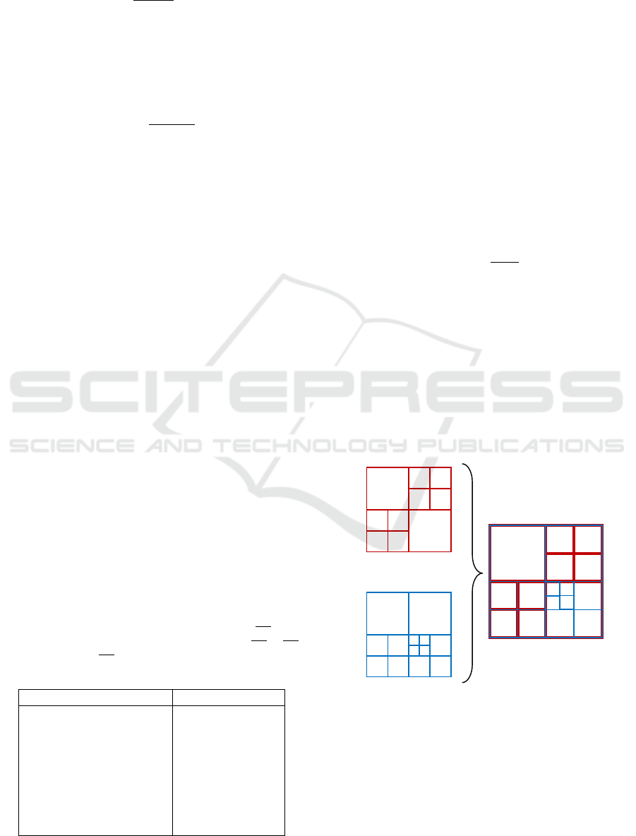
As tile selection runs independently for geom-

etry and texture, we end up having three cases of

geometry-texture tile correspondences: 1-to-1, n-to-

1, 1-to-n. Figure 5 illustrates these different corre-

spondence cases.

Geometry Quadtree

Texture Quadtree

Combined Quadtree

Figure 5: Correspondence among geometry (in red) and

texture (in blue) tiles: at the left quadrants, 1-to-1 corre-

spondence cases are conﬁgured; at the upper right quadrant,

there is a n-to-1 case and, at the lower right quadrant, there

is a 1-to-n case, which requires the use of virtual geometry

tiles to be rendered.

The 1-to-1 case is the direct one; we have one ge-

ometry tile for each texture tile: vertices deﬁning the

patches receive texture coordinates from 0.0 to 1.0.

GRAPP 2018 - International Conference on Computer Graphics Theory and Applications

244

The n-to-1 case is also simple: there are n geome-

try tiles mapped into one texture tile. Texture coordi-

nates are transformed accordingly, and all geometry

tiles uses the same texture object.

The 1-to-n case is the one that requires a more

elaborated solution: we have one geometry tile that

must be rendered using different texture objects. It

is needed to render the geometry tile multiple times,

one for each texture tile. We see two approaches for

doing this. In the ﬁrst approach, for each render pass,

we would select the patches covered by each texture

tile. Although this solution seems straightforward, it

presents two important drawbacks: (i) the correspon-

dence factor, n, would be limited by the number of

patches in a geometry tile; (ii) we would need a spe-

cialized algorithm to handle tiles with less patches.

We have opted for a second solution: we generate

a virtual geometry tile for each texture tile. Each vir-

tual tile is subdivided into the same number of patches

as a regular tile, so there is no need to modify the al-

gorithm. What differs is that a virtual tile uses a sub-

set of the elevation data: all virtual tiles are render-

ing using the same elevation data; texture coordinates

to access these data are assigned accordingly. Each

patch of virtual tiles inherits the object-space errors

annotated to the containing real patch.

6 RESULTS AND DISCUSSION

In this section, we describe a set of computational

experiments we used to test and tune the proposed

method. All experiments were run on a i7-3960X pro-

cessor computer with 24GB of RAM, equipped with

a NVIDIA Geforce GTX TITAN graphics card with

6GB of VRAM.

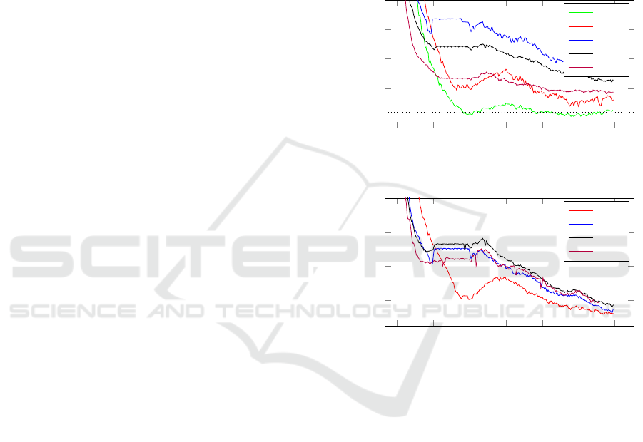
6.1 Tile and Patch Size Analysis

First, we analyze the inﬂuence of the geometry tile

size. For this computational experiment, we used a

high-resolution version of the Puget Sound Terrain.

The elevation data has a resolution of 65K × 65K

with 4 meter pixel spacing, using the aerial imagery

mapped as texture with 262K × 262K in size and 1

meter pixel spacing. The dataset was obtained from

(WU, 2017) and (USGS, 2017), totalizing 250GB of

disk space. We set the screen resolution to 1920 ×

1080 and the geometry error tolerance to 1.0 pixel.

To run the experiment, we deﬁned a camera path

over the terrain, crossing ﬂat and bumpy regions along

the way. We run the same experiment with two differ-

ent patch size (32 × 32 and 64 × 64) and tested differ-

ent tile sizes. Figures 6 and 7 show the achieved frame

rate. In this experiment, we got better performance

with 128 × 128 tiles for patches of 32 × 32 and with

256 × 256 tiles for patches of 64 × 64, what suggests

an ideal relation of 4 × 4 patches per tile on this ma-

chine. As we increase tile size, we reduce the height

of the quadtree, thus alleviating CPU workload and

increasing performance. On the other hand, as we in-

crease tile size, we reduce LOD granularity, requir-

ing more GPU memory and processing. Tests with

smaller patches resulted in worse performance.

100

150

200

250

Frame Rate

tile 32

tile 64

tile 128

tile 256

tile 512

Figure 6: Achieved frame rate along camera path for patch

size of 32 × 32.

100

150

200

250

Frame Rate

tile 64

tile 128

tile 256

tile 512

Figure 7: Achieved frame rate along camera path for patch

size of 64 × 64.

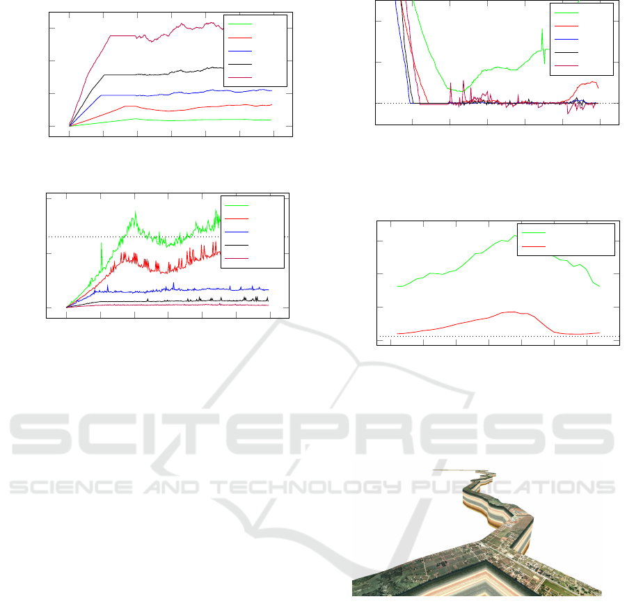
The following ﬁgures show different measure-

ments along the camera path for the 32 × 32 patch;

similar results were achieved for the 64 × 64 patch.

Figure 8 shows the required GPU memory for dif-

ferent tile sizes. The 128 × 128, which delivered

better performance, presents a good compromise be-

tween performance and requested memory resource.

Figure 9 shows the required CPU time to process

the frames along the camera way. As expected,

small tiles increases CPU workload, degrading per-

formance. Figure 10 shows the observed error in

screen space; recall that the used tolerance was set to

1 pixel. Small tiles do not honor the requested image

quality, since the application becomes CPU limited,

not being able to assure the quality in real time.

6.2 Comparison with Other Methods

We compared the rendering performance of our

method with the implementation of the chunked LOD

A Hybrid CPU-GPU Scalable Strategy for Multi-resolution Rendering of Large Digital Elevation Models with Borders and Holes

245

200

400

600

·10

#Memory

tile 32

tile 64

tile 128

tile 256

tile 512

Figure 8: Required GPU memory (in MB) per frame along

camera path (patch 32 × 32).

CPU Time

tile 32

tile 64

tile 128

tile 256

tile 512

Figure 9: Required CPU processing time (in milliseconds)

per frame along camera path (patch 32 × 32).

approach provided by (Ulrich, 2000). The available

code uses the Puget Sound data with 16k × 16k of

resolution. In the experiment, we set the screen er-

ror tolerance to one pixel and use a similar camera

paths. Figure 11 shows the achieved performance

along the camera path: our approach was in average

6.5x faster than the chunked LOD approach. This rel-

ative gain is higher than the one reported by (Yusov

and Shevtsov, 2011) but our experiment was ran on a

different equipment (they reported their proposal run

3.5x faster than the chunked LOD approach, using

two pixel tolerance on a NVidia GTX480).

6.3 Terrain Strip

In order to demonstrate the ability of our system to

handle terrain with irregular border, we run a sec-

ond experiment using a dataset that represents the el-

evation model of 1,000 kilometers of a terrain strip

that is the site a natural gas/oil pipeline, as shown

in Figure 12. This model is used in an application

to monitor emergency situations along the pipeline.

The raw dataset consists of several partially overlap-

ping terrain patches, one for each kilometer of the

pipe, resulting in 86 GB and 130 GB of elevation

and aerial imagery data, respectively. To pre-process

this dataset, we compose all ﬁles into a virtual raster

ﬁle, using a common GIS format (Virtual Raster).

The ﬁnal virtual image resolution was 2

. How-

ever, since this virtual image contains large amount

of void data, the pre-processing is performed in rea-

1.2

1.4

Screen Error(Max)

tile 32

tile 64

tile 128

tile 256

tile 512

Figure 10: Observed maximum screen space error (in pix-

els) per frame along camera path (patch 32 × 32). Recall

we request an error of at most 1 pixel; values above this

number signalize the system is not capable of delivering the

requested quality in real time.

500

1,000

1,500

Frame Rate

Our proposal

Ulrich’s approach

Figure 11: Comparison on performance of our approach

and the chunked LOD approach.

sonable time, only persisting tile with valid data. The

proposed system is capable of rendering such model

smoothly, from overview to zoom-in shots.

(a)

Figure 12: A rendered image of an actual terrain strip along

a gas/oil pipeline of 1,000 kilometers.

6.4 Seismic Surface

This last experiment demonstrates our system dealing

with internal holes in the surface. We used a horizon

surface resulted from an actual seismic data process-

ing. This surface is represented by an elevation model

but contains a large amount of void data, and correctly

rendering the holes is crucial for an accurate inter-

pretation of the model. Figure 13 shows a rendered

image. Again, the proposed system was capable of

rendering the model smoothly ensuring image quality

even for the complex structure of such a model.

GRAPP 2018 - International Conference on Computer Graphics Theory and Applications

246

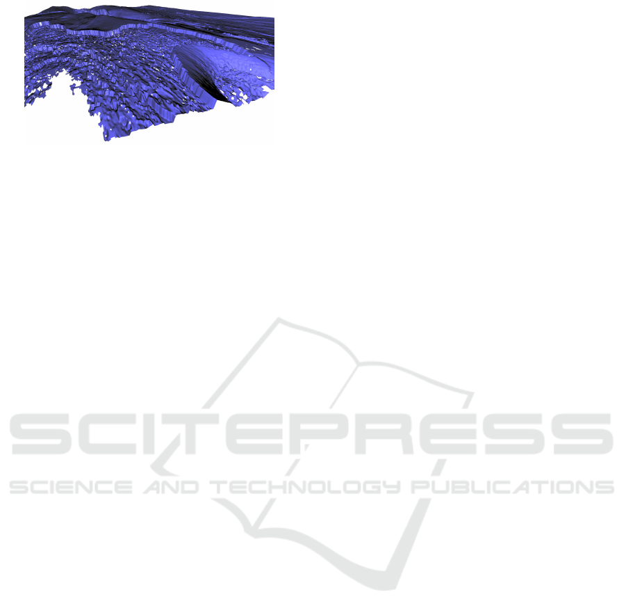
Figure 13: A rendered image of an actual horizon surface

from a seismic data.

7 CONCLUSION

We presented a new hybrid CPU-GPU strategy to ren-

der large digital elevation models with aerial imagery

mapped as textures. Level of detail managements,

for geometry (elevation) and texture (aerial imagery),

run independently. On the CPU, a multi-threaded

implementation is responsible for selecting, loading,

and transferring to the GPU active tiles. Geometry

tiles are decomposed into patches, and tessellation

shaders are used to determine tessellation levels for

each patch. The proposed method avoids crack be-

tween patch and tile interfaces by construction. Ge-

ometry and texture tiles are combined with no extra

data load, even in the case where one geometry tile is

covered by a set of different texture tiles.

We also extended the proposal for handling terrain

with irregular borders and surfaces with holes, intro-

ducing the concept of horizontal errors. Dealing with

irregular borders mitigates the constraint of power of

two (plus one for the border) on terrain dimensions;

supporting surfaces with hole has an important ap-

plication on rendering interpreted seismic surfaces of

large datasets.

ACKNOWLEDGEMENTS

We thank CNPq (Brazilian National Council for Sci-

entiﬁc and Technological Development) and Petro-

bras (the Brazilian oil company) for the ﬁnancial sup-

port to conduct this research.

REFERENCES

Cervin, A. (2012). Adaptive Hardware-accelerated Ter-

rain Tessellation. PhD thesis, Linköpings Universitet,

Tekniska Högskolan.

Cignoni, P., Ganovelli, F., Gobbetti, E., Marton, F., Pon-

chio, F., and Scopigno, R. (2003a). BDAM —

Batched Dynamic Adaptive Meshes for High Perfor-

mance Terrain Visualization. Computer Graphics Fo-

rum, 22(3):505–514.

Cignoni, P., Ganovelli, F., Gobbetti, E., Marton, F., Pon-

chio, F., and Scopigno, R. (2003b). Planet-Sized

Batched Dynamic Adaptive Meshes (P-BDAM). In

Proceedings of the 14th IEEE Visualization 2003

(VIS’03), VIS ’03, pages 20–, Washington, DC, USA.

IEEE Computer Society.

Duchaineau, M., Wolinsky, M., Sigeti, D., Miller, M.,

Aldrich, C., and Mineev-Weinstein, M. (1997).

ROAMing terrain: Real-time Optimally Adapting

Meshes. In Visualization ’97., Proceedings, pages 81–

88.

Fernandes, A. and Oliveira, B. (2012). Gpu tessellation:

We still have a lod of terrain to cover. In Cozzi, P. and

Riccio, C., editors, OpenGL Insights, pages 143–160.

CRC Press.

Kang, H., Jang, H., Cho, C.-S., and Han, J. (2015). Multi-

resolution Terrain Rendering with GPU Tessellation.

Vis. Comput., 31(4):455–469.

Lindstrom, P., Koller, D., Ribarsky, W., Hodges, L. F.,

Faust, N., and Turner, G. A. (1996). Real-time, contin-

uous level of detail rendering of height ﬁelds. In Pro-

ceedings of the 23rd annual conference on Computer

graphics and interactive techniques, pages 109–118.

ACM.

Lindstrom, P. and Pascucci, V. (2001). Visualization of

large terrains made easy. In Visualization, 2001.

VIS’01. Proceedings, pages 363–574. IEEE.

Losasso, F. and Hoppe, H. (2004). Geometry Clipmaps:

Terrain Rendering Using Nested Regular Grids. In

ACM SIGGRAPH 2004 Papers, SIGGRAPH ’04,

pages 769–776, New York, NY, USA. ACM.

Pajarola, R. and Gobbetti, E. (2007). Survey of semi-regular

multiresolution models for interactive terrain render-

ing. The Visual Computer, 23(8):583–605.

Schäfer, H., sner, M. N., Keinert, B., Stamminger, M., and

Loop, C. (2014). State of the Art Report on Real-time

Rendering with Hardware Tessellation. In Eurograph-

ics, pages 93–117.

Ulrich, T. (2000). Rendering massive terrains using chun-

ked level of detail. ACM SIGGRAPH Course “Super-

size it! Scaling up to Massive Virtual Worlds”.

USGS (2017). US geological survey - USGS.

https://www.usgs.gov/products/maps/gis-data.

WU, G. R. G. (2017). Geomorphological re-

search group - washington university.

http://gis.ess.washington.edu/data/.

Yusov, E. and Shevtsov, M. (2011). High-performance ter-

rain rendering using hardware tessellation. Journal of

WSCG, 19(3):85–92.

A Hybrid CPU-GPU Scalable Strategy for Multi-resolution Rendering of Large Digital Elevation Models with Borders and Holes

247