
Fiber Cable Network Design with
Operations Administration & Maintenance Constraints
Vincent Angilella
1,2
, Matthieu Chardy
1
and Walid Ben-Ameur
2
1
Orange Labs, 40-44 Avenue de la Republique, 92320, Chatillon, France
2
SAMOVAR, Telecom SudParis, CNRS, Paris-Saclay University, 9 Rue Charles Fourier, 91011 Evry Cedex, France
Keywords:
Optical Networks, Network Design, Mixed Integer Programming, Dynamic Programming.
Abstract:
We introduce two specific design problems of optical fiber cable networks that differ by a practical mainte-
nance constraint. An integer programming based method including valid inequalities is introduced for the
unconstrained problem. We propose two exact solution methods to tackle the constrained problem: the first
one is based on mixed integer programming including valid inequalities while the second one is built on dy-
namic programming. The theoretical complexities of both problems in several cases are proven and compared.
Numerical results assess the efficiency of both methods in different contexts including real-life instances, and
evaluate the effect of the maintenance constraint on the solution quality.
1 INTRODUCTION
Fiber To The Home (FTTH) networks are currently
deployed by telecommunications operators, and re-
quire a huge capital expenditure (see (Europe, 2016),
it can cost several billion euros to connect one mil-
lion households). The technological architecture cho-
sen by a majority of operators is to deploy passive
optical networks, which are based on passive optical
splitters. A passive optical splitter connects several
fibers on one of its sides to one at the other side (di-
vides or gathers the signal depending on its origin),
which leads to a tree topology of the FTTH networks
(illustrated in Fig. 1). The design of such networks
includes to decide the splitter locations, the civil en-
gineering infrastructure used (see (Bley et al., 2013),
(Chardy et al., 2013), (Gollowitzer et al., 2013), (Con-
treras and Fernandez, 2012)). Finally, the fiber cable
network has to be designed to connect these equip-
ment (see Fig. 1). These decisions are usually taken
in different steps.
This paper focuses on the problem of fiber cable
network design. This problem is highlighted in the
survey (Gr
¨
otschel et al., 2013) as an incomplete field
of study, especially when cable separation techniques
are considered. The work from (Angilella et al., 2016)
tackles the issue including the selection of civil engi-
neering infrastructure, but faces computational limits
on real-life instances. The paper (Mateus et al., 2000)
excludes weld costs, which are a significant expense
source. The work from (Angilella et al., 2017) deals
with the issue of cable backfeed, specific to the prob-
lem, but restricts the possible ways to serve the de-
mand. In the following we include several ways to
serve the demand (with fiber cables or fiber modules),
and introduce a maintenance constraint which, to our
knowledge, is novel.
The next section introduces two problems which
differ by the introduction of an Operation Adminis-
tration & Maintenance constraint. We introduce an al-
gorithm based on integer programming for the uncon-
strained problem in Section 3.1. Two solution meth-
ods are then proposed for the constrained problem, an
integer programming based solution in Section 3.2,
and a dynamic programming based solution in Sec-
tion 4. The theoretical complexities of the problems
are argued in Section 5. All solution methods are as-
sessed numerically in Section 6.
2 PROBLEM DESCRIPTION
The general problem tackled in this paper consists
in connecting one splitter location to several client
groups, using fiber cables, with minimal cost. It arises
several times in a given FTTH network, notably once
for each splitter location.
94
Angilella, V., Chardy, M. and Ben-Ameur, W.
Fiber Cable Network Design with Operations Administration & Maintenance Constraints.
DOI: 10.5220/0006621700940105
In Proceedings of the 7th International Conference on Operations Research and Enterprise Systems (ICORES 2018), pages 94-105
ISBN: 978-989-758-285-1
Copyright © 2018 by SCITEPRESS – Science and Technology Publications, Lda. All rights reserved
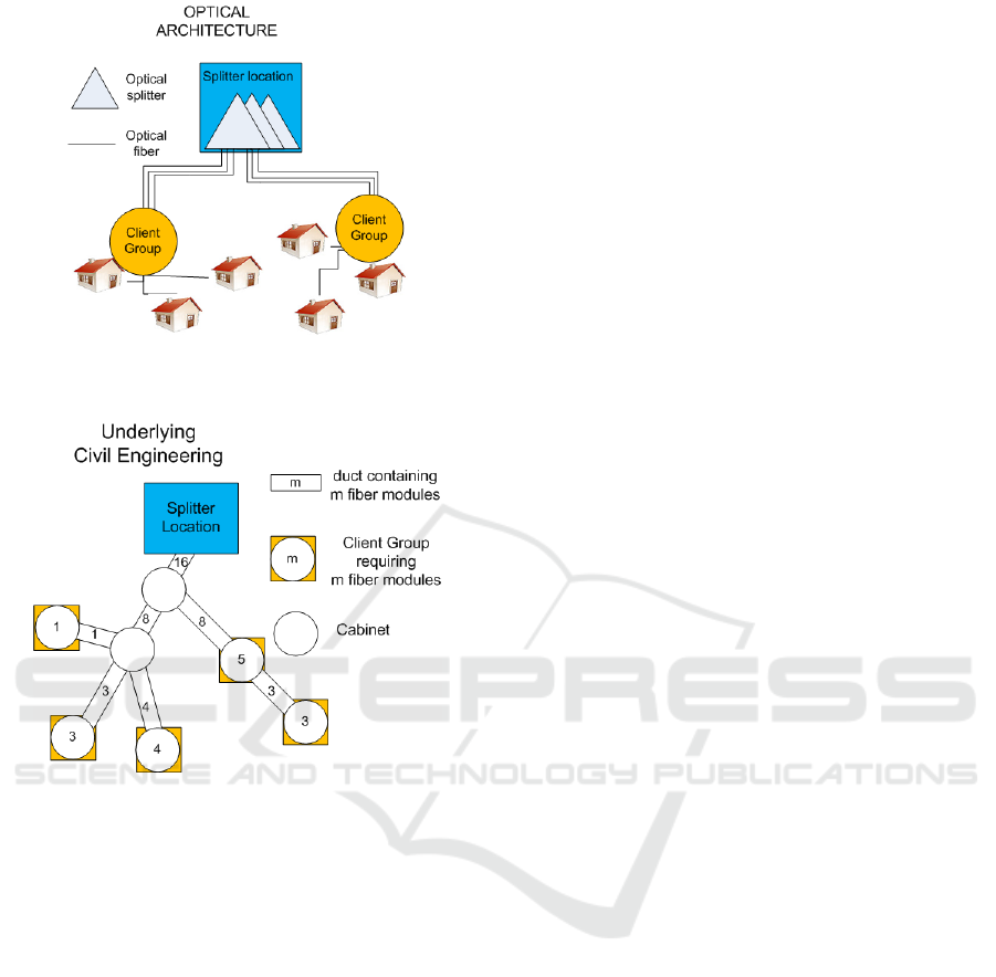
Figure 1: Underlying optical architecture example. It has
a tree topology; the splitter location is connected to every
client group.
Figure 2: Underlying civil engineering tree example. The
ducts, cabinets, demands and number of fiber modules are
known.
2.1 Unconstrained Problem
Cables are to be laid out in a civil engineering in-
frastructure (usually the one used for the legacy cop-
per network) with a tree topology, assumed chosen
within previous decision steps. The cables have an
arborescent structure from the splitter location to the
client groups. Along the ducts of this infrastructure
are located street cabinets, in which the demand lies.
The civil engineering structure used is supposed to be
known due to previous decision making, as well as the
demand in each cabinet.
Fiber cables contain several fiber modules, and
each fiber module contains several fibers. Due to op-
erational constraints, modules are not dividable, and
all modules on a given network are supposed to be
identical. This allows us to consider only fiber mod-
ules, and ignore the fiber level. Some of the mod-
ules are connected to the fiber source on one of their
ends, and on the fiber demand on the other end. These
are actually used, and are called ”active modules”, the
other ones are called ”dead modules”. The latter can
arise due to cables not matching exactly the demand
or in the operations described below (example: a 4
module cable serving a cabinet which requires 3 mod-
ules). Since all the demand is known and there is only
one path from the source to a given demand point,
the number of active modules that must be deployed
through a given duct is known (see Fig 2).
At a cabinet, cables can endure a splicing opera-
tion, which leads to two basic configurations (see Fig.
3):
• All cables are continued. One only has to pay for
the cost of laying out cables.
• One cable is spliced. It is cut at the cabinet, and
its active modules are welded to active modules of
new cables, referred to as ”born cables”. A protec-
tive box, the size of which depends on the spliced
cable size, is installed. One has to pay for the ca-
bles, the box and the welds.
There are two different ways to serve the demand
that cannot be combined (see Fig. 4):
• Cable-served. In this case, a single cable brings
all the required active modules to the demand cab-
inet.
• Module-served. In this case, a splicing operation
is done in the cabinet, and some modules from the
spliced cable are used to serve the demand. No
welds are done on these modules.
Additional engineering rules have to be taken into
account:
• At most one cable can be spliced at a street cab-
inet. This is due to space restrictions and regula-
tory constraints (protective boxes are large).
• The demand of a given cabinet must be served by
at most one cable.
The cost elements are as follows:
• The cost of a cable is linear with respect to its
length, and concave with respect to its size (i.e.
its number of modules). This derives from the
catalogues of cable manufacturers, who propose
a fixed price per length unit for each cable size.
• The cost of a protective box depends on the size
of the cable being spliced. It is a piecewise con-
stant function. This derives from the number of
different boxes sold by manufacturers.
• The cost of welds depends on the number of welds
to be done in a given cabinet. It is piecewise linear
concave, and derives from manpower cost consid-
erations.
Fiber Cable Network Design with Operations Administration & Maintenance Constraints
95

Figure 3: Left: Continued cables; Right: Splicing operation.
Figure 4: Left: Module-served demand node; Right: Cable-
served demand node.
This decision problem, referred to as FCNDA
(Fiber Cable Network Design in an Arborescence) in
the following, can be formulated as follows: given a
civil engineering arborescence, demand nodes, a set
of available cables and the associated costs, design a
minimum cost optical fiber cable network satisfying
the engineering rules listed above.
Section 2.2 introduces a restriction of the FCNDA
problem.
2.2 Constrained Problem
We restrict the problem by imposing that all cables
going through a given duct are born in the same cab-
inet (eventually the fiber source). This restriction is
illustrated in Fig. 5. It is motivated by operations and
maintenance considerations. Indeed, assuming all the
cables of a given duct are damaged, then an interven-
tion has to be done at the cabinets where each of these
cables is born. If the rule is respected, an intervention
is necessary in only one cabinet.
The constrained decision problem, referred to as
EFCNDA (Easy-maintenance Fiber Cable Network
Design in an Arborescence) in the following consists
in designing a FCNDA solution where cables on a
same duct are born in the same cabinet with minimal
cost.
3 INTEGER PROGRAMMING
3.1 FCNDA
3.1.1 Notation and Formulation
The following notation will also be used in section 4.
An arborescence G = (V, A) describes the civil
engineering infrastructure, V the cabinets and A the
ducts, and its root r ∈ V denotes the fiber source.
For any i ∈ V, D
i
∈ N denotes the demand (number
of active modules required) in node i. We define
V
∗
= V \ {r}. The set of demand nodes is noted
V
D
= {v ∈ V, D
v
> 0}, the set of nodes without de-
mand V
N
= V
∗
\V
D
. Each arc (i, j) ∈ A has a length
d
i, j
and must contain m
act
i, j
active modules. For i ∈ V ,
let Γ
+
(i) denote the set of successors of i and let γ(i)
be its predecessor.
The set of cable types is denoted by L = {1, ..,L}
where L is the number of different cable types avail-
able. Cables of type l ∈ L have a size of M
l
∈ N mod-
ules, and for l ∈ L, we denote M
l
= {1, .., M
l
} the
range of possible number of active modules in a cable
ICORES 2018 - 7th International Conference on Operations Research and Enterprise Systems
96
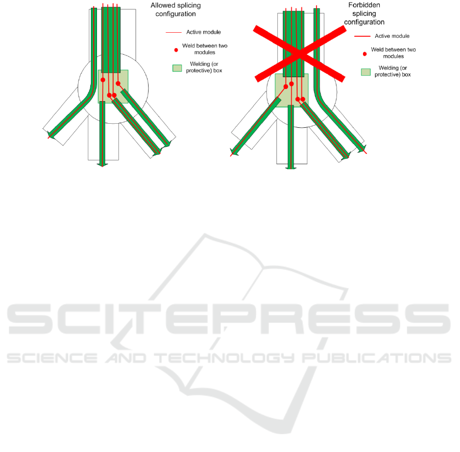
Figure 5: Left: Allowed splicing configuration for EFCNDA. On all edges, cables are born in the same cabinet; Right:
Forbidden splicing configuration for EFCNDA. On the bottom-right duct, two different cables are born in different cabinets.
of type l. The cable sizes (M
l
)
l
are supposed to be
ordered with respect to l. The largest cable has a size
of M
L
, which corresponds to the maximal number of
welds done in a node.
For l ∈ L, let us define C
le
l
the cost per length unit
of a cable of type l, and PB
l
the cost of a box of type l.
For m ∈ {0, .., M
L
}, let us define the cost of the small-
est cable able to contain m active modules C
min
m
= C
le
l
1
where l
1
= min{l ∈ L, m ≤ M
l
} (which is also the
cheapest as cable costs are increasing with respect to
the cable size), and PW
m
the cost for welding m mod-
ules.
We introduce P the set of oriented paths of G, and
for p ∈ P , we denote by s(p) its source node, t(p) its
target node, and d
p
its length (which extends d from
A to P ).
We define the following variables:
• ∀l ∈ L, ∀p ∈ P , k
spl
p,l
∈ {0, 1} the binary variable
equal to 1 iff there is a cable of size l on path p
spliced in t(p).
• ∀p ∈ P ,k
dem
p
∈ {0, 1} the binary variable equal to
1 iff there is a cable on path p serving the demand
in t(p) in a cable-served way; its type is known, it
is min{l ∈ L |M
l
≥ D
t(p)
}.
• ∀p ∈ P , m
spl
p
∈ {0, .., M
L
} the number of active
modules of the cable on path p spliced in t(p).
• ∀i ∈ V
∗
, ∀m ∈ M
L
, w
i,m
the binary variable equal
to 1 iff m welds are done in node i.
The problem can be formulated as follows:
min
∑
p∈P
d
p
·
∑
l∈L
(C
le
l
· k
spl
p,l
) +C
min
D
t(p)
· k
dem
p
!
+
∑
i∈V
N
∑
m∈M
L
PW
m
· w
i,m
+
∑
p∈P
∑
l∈L
PB
l
· k
spl
p,l
such that
∀i ∈ V
∗
,
∑
p∈P |t(p)=i
∑
l∈L
k
spl
p,l
≤ 1 (1)
∀i ∈ V
D
,
∑
p∈P |t(p)=i
k
dem
p
≤ 1 (2)
∀p ∈ P ,
∑
l∈L
M
l
· k
spl
p,l
≥ m
spl
p
(3)
∀i ∈ V
∗
,
∑
p∈P |t(p)=i
m
spl
p
=
D
i
· (1 −
∑
p∈P |t(p)=i
k
dem
p
)
+
∑
p∈P |s(p)=i
(m
spl
p
+ D
t(p)
k
dem
p
) (4)
∀i ∈ V
∗
,
∑
m∈M
L
m · w
i,m
=
∑
p∈P |i=s(p)
(m
spl
p
+ D
t(p)
· k
dem
p
) (5)
∀i ∈ V
N
,
∑
m∈M
L
w
i,m
≤ 1 (6)
k
dem
∈ {0, 1}
|P |
, k
spl
∈ {0,1}
|P |×L
,
w ∈ {0, 1}
|V
∗
|×M
L
, m
spl
∈ {0,.., M
L
}
|P |
.
In the cost function, the first term stands for the
cost of cables, the second term for the cost of welds,
and the last term for the cost of boxes. Equations
(1) ensure that at most one cable is spliced in a node.
Constraints (2) state that at most one cable serves the
demand in a cable-served way. Equations (3) make
sure that spliced cables are large enough to contain
their number of active modules. Constraints (4) are
active module conservation equations. The left-hand
side term stands for the number of modules of the
spliced cable. The first right-hand side term is the
number of modules necessary to serve the demand, in
Fiber Cable Network Design with Operations Administration & Maintenance Constraints
97

case it is not cable-served. The last term is the number
of active modules of born cables. Finally, constraints
(5) and (6) ensure that w counts the number of welds
to be done in each node.
Remark 3.1. It is possible to fix the value of some
variables. First, notice that leaf nodes are demand
nodes. These nodes will be served in a cable-served
way, and no operation will be done inside them. This
gives, for all nodes i ∈ V
D
such that |Γ
+
(i)| = 0:
∀m ∈ M
L
, w
i,m
= 0
∀p ∈ P |t(p) = i, ∀l ∈ L , k
spl
p,l
= 0
Furthermore, the number of welds done in a node
cannot exceed the number of active modules going out
of this node. This gives:
∀i ∈ V
∗
, ∀m ∈ M
L
, m >
∑
j∈Γ
+
(i)
m
act
i, j
=⇒ w
i,m
= 0
3.1.2 Valid Inequalities
We propose here several valid inequalities to tighten
the linear programming continuous relaxation the for-
mulation.
Let us define, for all m ∈ N, the minimum cost
per length unit of a set of cables able to contain m
active modules denoted by LB(m). For a given m,
LB(m) = {min
∑
l∈L
C
le
l
·n
l
|
∑
l∈L
M
l
·n
l
≥ m, n ∈ N
L
}.
The following inequalities are valid for the FCNDA
problem:
∀(i, j) ∈ A,
∑
p∈P |(i, j)∈p
∑
l∈L
(C
le
l
· k
spl
p,l
) +
C
min
D
t(p)
· k
dem
p
≥ LB(m
act
i, j
) (7)
The left hand side is the cost per length unit of the
cables going through arc (i, j).
Let us consider a path p ∈ P such that t(p) ∈ V
D
and s(p) 6= r. If there is a cable deployed on p, born
in s(p) and serving the demand in t(p), then we know
that there is a splicing operation done in s(p). Fur-
thermore, there are at least D
t(p)
welds in this opera-
tion, since the cable serving t(p) contains D
t(p)
active
modules. This gives the following valid inequalities
for the FCNDA problem:
∀p ∈ P |t(p) ∈ V
D
and s(p) 6= r,
k
dem
p
≤
∑
m≥D
t(p)
w
s(p),m
(8)
3.2 EFCNDA
EFCNDA can be solved by using the same variables
as in Section 3.1. The cost function is the same, the
set of feasible solutions is described by constraints (1)
to (6) to which we add the maintenance constraints
described below:
∀(p, p
0
) ∈ P
2
such that s(p) 6= s(p
0
)
and ∃a ∈ A, a ∈ p, a ∈ p
0
k
dem
p
+ k
dem
p
0
≤ 1 (9)
∑
l∈L
k
spl
p,l
+
∑
l∈L
k
spl
p
0
,l
≤ 1 (10)
∑
l∈L
k
spl
p,l
+ k
dem
p
0
≤ 1 (11)
These constraints ensure that on two paths which
have different origins but an edge in common, there
can be only one cable.
The next section introduces an alternative mixed
integer programming approach for EFCNDA, based
on arcs rather than paths. It uses the properties of the
problem, and has less variables and less constraints.
3.2.1 Notation and Formulation
We keep the same notation for the problem instance.
In addition, let us define for (i, j) ∈ A,U
i, j
an upper
bound of the cost per length unit of the cables going
through (i, j).
We define the following variables:
• ∀(i, j) ∈ A, x
i, j
∈ {0, 1} the binary variable equal
to 1 iff the cables on edge (i, j) are born in i.
• ∀(i, j) ∈ A, c
i, j
∈ R the continuous variable equal
to the cost per length unit of the cables on edge
(i, j) (when all constraints are satisfied, including
integrality constraints).
• ∀(i, j) ∈ A, z
i, j
∈ R the continuous variable equal
to x
i, j
· c
i, j
.
• ∀i ∈ V
D
, u
i
∈ {0, 1} the binary variable equal to 1
iff the node i is module-served.
• ∀i ∈ V
∗
, ∀m ∈ M
L
, w
i,m
the binary variable equal
to 1 iff m welds are done in node i (since its mean-
ing is identical to Section 3.1, we keep the same
name).
• ∀i ∈ V
∗
, ∀l ∈ L, y
i,l
the binary variable equal to 1
iff a cable of size l is spliced in i.
The problem can be formulated as follows:
min
∑
i∈V
∗
∑
m∈M
L
PW
m
· w
i,m
+
∑
(i, j)∈A
d
i, j
· c
i, j
+
∑
i∈V
∗
∑
l∈L
PB
l
· y
i,l
such that ∀i ∈ V
D
,
ICORES 2018 - 7th International Conference on Operations Research and Enterprise Systems
98

c
γ(i),i
=
∑
l∈L
C
le
l
y
i,l
+
∑
j∈Γ
+
(i)
c
i, j
−
∑
j∈Γ
+
(i)
z
i, j
+ (1 − u
i
) ·C
min
D
i
(12)
∀i ∈ V
N
, c
γ(i),i
=
∑
l∈L
C
le
l
y
i,l
+
∑
j∈Γ
+
(i)
c
i, j
−
∑
j∈Γ
+
(i)
z
i, j
(13)
∀i ∈ V
D
,
∑
l∈L
M
l
· y
i,l
≥
D
i
· u
i
+
∑
j∈Γ
+
(i)
m
act
i, j
· x
i, j
(14)
∀i ∈ V
∗
,
∑
l∈L
M
l
· y
i,l
≥
∑
j∈Γ
+
(i)
m
act
i, j
· x
i, j
(15)
∀i ∈ V
∗
,
∑
l∈L
y
i,l
≤ 1 (16)
∀i ∈ V
∗
,
∑
m∈M
L
m · w
i,m
=
∑
j∈Γ
+
(i)
m
act
i, j
· x
i, j
(17)
∀i ∈ V
∗
,
∑
m∈M
L
w
i,m
≤ 1 (18)
∀(i, j) ∈ A, z
i, j
≥ c
i, j
−U
i, j
· (1 − x
i, j
) (19)
∀(i, j) ∈ A, z
i, j
≤ U
i, j
· x
i, j
(20)
∀(i, j) ∈ A, z
i, j
≤ c
i, j
(21)
u ∈ {0, 1}
|V
D
|
, w ∈ {0, 1}
|V
∗
|×M
L
,
x ∈ {0, 1}
|A|
, y ∈ {0, 1}
|V
∗
|×L
,
c ∈ R
|A|
, z ∈ R
|A|
.
The first term of the cost function denotes the cost
of welds, the second term stands for the cost of ca-
bles, and the last term stands for the cost of boxes.
Equations (12) ensure that the cost per length unit of
any arc is properly counted. The term
∑
l∈L
C
le
l
y
i,l
stands for the cost of the cable spliced in i, if any.
If for some arc (i, j) ∈ A such that j ∈ Γ
+
(i) we have
x
i, j
= 0, then the cables on arc (i, j) come from arc
(γ(i), i) unchanged. Otherwise, they come from the
splicing operation done in i. The last term stands for
the cost of the cable serving the demand in i. Equa-
tions (13) are the equivalent concerning nodes without
demand. Equations (14), (15) and (16) ensure that the
cable spliced in i is large enough to contain its active
modules. The first term of the right-hand side of (14)
stands for modules serving the demand, the second
term for modules of born cables. Constraints (17) and
(18) ensure that the variable w
i,m
is equal to 1 iff there
are m welds done in node i. Finally, constraints (19),
(20) and (21) ensure that ∀(i, j) ∈ A, z
i, j
= x
i, j
· c
i, j
(these are Mc Cormick linearisation equations).
Remark 3.2. It is possible to fix the value of some
variables. Assuming there exists i ∈ V
∗
and m
1
∈
M
L
such that w
i,m
1
= 1, then by (17), we know that
there exists S ⊆ Γ
+
(i) such that m
1
=
∑
j∈S
m
act
i, j
.
This gives by contraposition ∀i ∈ V
∗
, ∀m ∈ M
L
if
m 6∈ {
∑
j∈S
m
act
i, j
|S ⊆ Γ
+
(i)} then w
i,m
= 0. It can be
computed either in O(2
|Γ
+
(i)|
) or in O(|Γ
+
(i)| × M
L
)
(which is not a polynomial with respect to the instance
size, provided M
L
is not coded in an unary system).
3.2.2 Valid Inequalities
The continuous relaxation of the formulation above
does not seem to be very tight in practice (see Table
4 from Section 6). We propose here several valid in-
equalities to tighten the continuous relaxation of the
formulation.
In nodes without demand, if a cable of size l is
spliced, then it has a number of active modules be-
tween M
l
and M
l−1
+ 1; otherwise one could install a
smaller cable and obtain a cheaper solution. With the
convention M
0
= 0 and M
0
=
/
0, every optimal solu-
tion of the EFCNDA problem verifies the following:
∀i ∈ V
N
, ∀l ∈ L , y
i,l
=
∑
m∈M
l
\M
l−1
w
i,m
(22)
With a reasoning similar to the one from 3.1.2 (see
definition of LB), we can get a lower bound of the cost
per length unit of the cables on each arc. The follow-
ing inequalities are valid for the EFCNDA problem:
∀(i, j) ∈ A, c
i, j
≥ LB(m
act
i, j
) (23)
If the cables on some arc (i, j) ∈ A are born in
i, then at least m
act
i, j
welds are done in node i. This
implies that the following inequalities are valid for the
EFCNDA problem.
∀(i, j) ∈ A, x
i, j
≤
∑
m∈M
L
|m≥m
act
i, j
w
i,m
(24)
4 DYNAMIC PROGRAMMING
FOR EFCNDA
For any node i ∈ V
∗
, we introduce the additional no-
tation V
pr
(i), which refers to the set of nodes on the
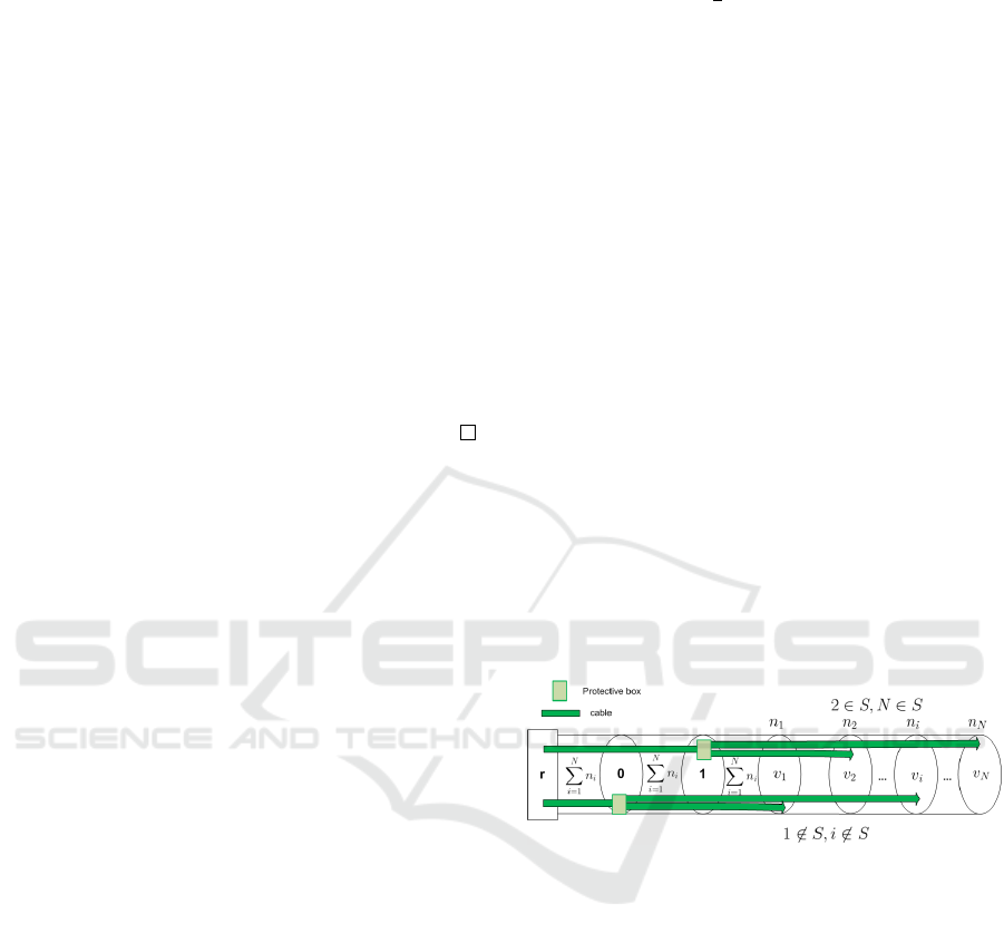
path from the root to i, excluding i and including r.
The EFCNDA problem can be solved by Algo-
rithm 1. To each node i ∈ V
∗
, and for each node
j ∈ V
pr
(i), we associate to i a label < j,C(i, j) >∈
V
pr
(i) × R where C(i, j) is the minimum cost of the
Fiber Cable Network Design with Operations Administration & Maintenance Constraints
99

Algorithm 1: Exact Resolution Algorithm for EFCNDA.
1: procedure INITIALISATION()
2: for i ∈ V
D
|Γ
+
(i) =
/
0 do
3: for j ∈ V
pr
(i) do
4: Add to i the label < j,C
min
D
i
· d
p
> where p ∈ P is the only path s.t. s(p) = j and t(p) = i.
5: end for
6: Declare i labeled.
7: end for
8: end procedure
9: procedure RECURSION()
10: while ∃r
0
∈ Γ
+
(r) such that r
0
has not been labeled do
11: for every node i ∈ V
∗
such that all nodes in Γ
+
(i) have been labeled do
12: for j ∈ V
pr
(i) do
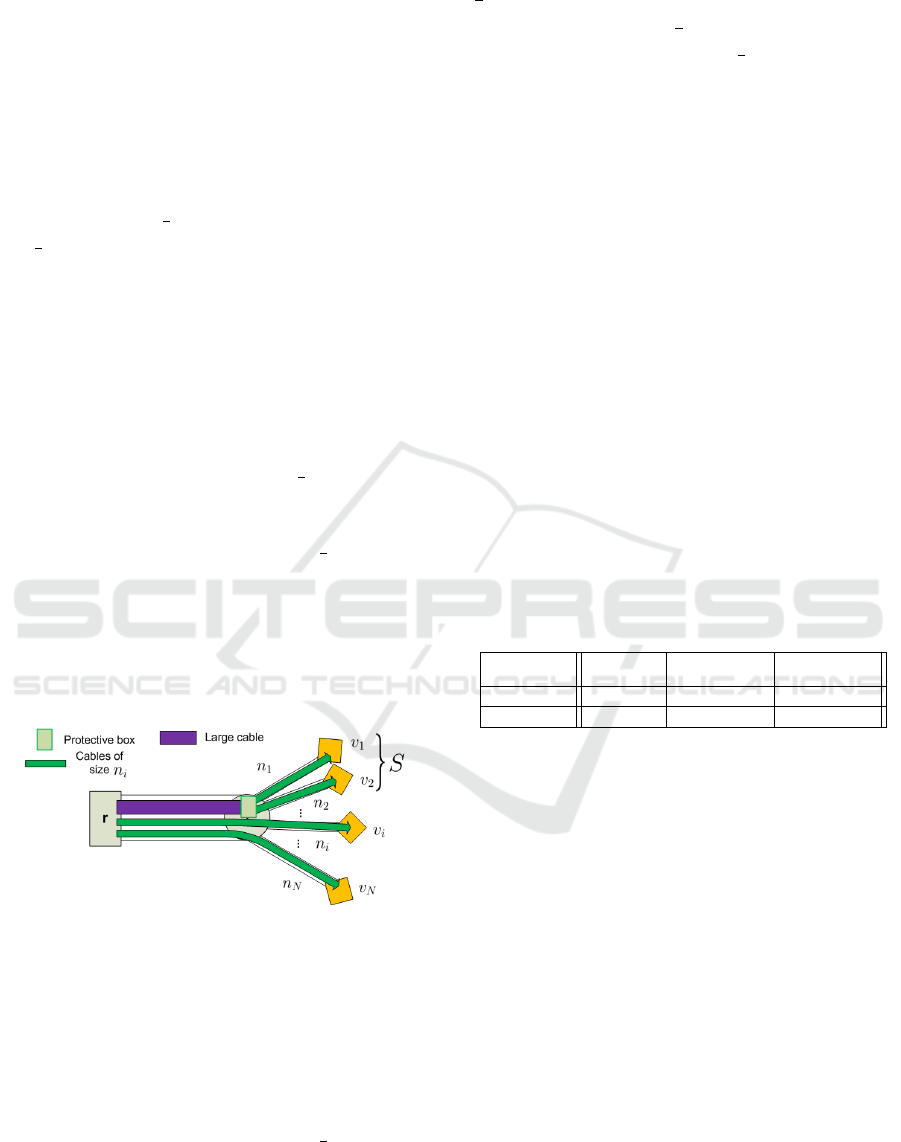
13: We select the operation in i minimizing the network cost.
14: Add the label < j,C(i, j) > to node i where
C(i, j) = min
S⊆Γ
+
(i),b∈{0,1}
∑
k∈S
C(k, i) +
∑
k∈Γ
+
(i)\S
C(k, j)
+PW
m
+ d
p
·C
le
l
1
+ d
p
·C
min
D
i
· (1 − b) (25)
with
m =
∑
k∈S
m
act
i,k
;l
1
= min{l ∈ L |M
l
≥ b · D
i
+
∑
k∈S
m
act
i,k
}
p ∈ P is the only path such that s(p) = j,t(p) = i
15: end for
16: Declare i labeled.
17: end for
18: end while
19: end procedure
20: procedure TERMINATION()
21: return
∑
r
0
∈Γ
+
(r)
C(r
0
, r)
22: end procedure
network rooted in i plus the cost of the cables on the
path from j to i, assuming these are born in node j.
The algorithm is initialized at leaf nodes (line 4),
which are cable-served demand nodes, and where the
size of the cable serving the demand is known.
For a node i such that all nodes in Γ
+
(i) have been
labeled, and for j ∈ V
pr
(i), (25) computes the mini-
mum cost operation if the next operation is done in j.
For i ∈ V
∗
and k ∈ Γ
+
(i), k ∈ S iff the cables going
through arc (i, k) are born in node i. Similarly, the
boolean b is equal to 1 iff the node i is module-served
(its meaning is similar than the variable u
i
in Section
3.2).
We propose to compute it with a brute-search al-
gorithm on the set S and on b. For given nodes i ∈
V
∗
, j ∈ V
pr
(i), it can be done in O(P
∗
(ln(M
L
), L) ×
2
|Γ
+
(i)|+1
) where P
∗
is a time sufficient to compute C
∗
(sums and minimums can be computed in polynomial
time).
Lemma 4.1. Algorithm 1 runs in time
O(P
∗
(ln(M
L
), L) × 2
maxΓ
× |V |
2
) where maxΓ
denotes the maximal degree (number of successors)
of a node in the graph and P
∗
is a polynomial.
Indeed, in each loop a number of iterations smaller
than V
∗
is done.
Proposition 4.2. Let us consider i ∈ V
∗
. When i is
declared labeled in algorithm 1, there exists a node
j ∈ V
pr
(i) such that in the label < j,C(i, j) >, C(i, j)
describes the cost of the minimum cost network in the
arborescence rooted in node i plus the cost of the ca-
bles on the path from j to i.
This proposition shows the validity of the algo-
rithm. We will start to prove it for leaf nodes, then
recursively on higher nodes.
Proof. Let us consider a leaf node i. In the mini-
mum cost network, it is served in a cable-served way
with a cable of type l
1
= min{l ∈ L |M
l
≥ D
i
}. This
cable is born in some node j ∈ V
pr
(i), eventually the
root. The minimum cost network has a cost 0 in
the arborescence rooted in j. Let us call p ∈ P the
only path such that s(p) = j and t(p) = i. The label
< j,C(i, j) > of i has a cost of C
min
D
i
· d
p
.
ICORES 2018 - 7th International Conference on Operations Research and Enterprise Systems
100
Let us consider a non-leaf node i ∈ V
∗
such that
all nodes in Γ
+
(i) have been labeled. In the minimal
cost network, the cables going through arc (γ(i), i) are
all born in a node j ∈ V
pr
(i). Thanks to the main-
tenance constraint, we know that they are all born
in the same node. Since all nodes k ∈ Γ
+
(i) have
been labeled, for each of these nodes, there is a node
j
k
∈ V
pr
(k) such that in the label < j
k
,C(k, j
k
) >,
C(k, j
k
) describes the cost of the minimum cost net-
work in the arborescence rooted in k plus the cost of
the cables on the path from j
k
to k. Furthermore, since
the cables going through arc (γ(i), i) are all born in j,
we have either j
k
= j or j
k
= i. Let us consider the
label < j,C(i, j) > of node i. If in the minimal net-
work i is module-served, then we will have b = 0 in
the computation of (25). Furthermore, let us consider
k ∈ Γ
+
(i). If j
k
= i, we will have k ∈ S in the compu-
tation of (25), and k ∈ Γ
+
(i) \ S otherwise. Hence the
result.
The termination of the algorithm derives from
Proposition 4.2. For each node r
0
∈ Γ
+
(r), we have
V
pr
(r
0
) = {r}. This implies, using this proposition,
that in the label < r,C(r
0
, r) >, C(r
0
, r) is the cost of
the minimum network cost in the arborescence rooted
in r
0
plus the cost of the cables on (r, r
0
). Summing
these values gives the minimum network cost.
The next section assesses the complexity of FC-
NDA and EFCNDA.
5 COMPLEXITY
We show in Section 5.1 that FCNDA is NP-hard even
with 1 cable size and an upper bound on the node de-
gree of 2, and in Section 5.2 that EFCNDA is NP-
hard.
5.1 FCNDA
Let us consider the Number Partitioning Problem
(NPP), which is shown to be NP-complete in (Karp,
1972).
Instance: A set of N strictly positive integers {n
i
∈
N|i ∈ {1, .., N}}.
Question: Is there a subset S ⊆ {1, ..,N} such that
∑
i∈S
n
i
=
∑
i6∈S
n
i
?
We consider an instance of the NPP and reduce
it to the following FCNDA instance. Let G = (V, A)
be an arborescence describing the civil engineer-
ing structure, (V = {r, 0, 1} ∪ {v
i
|i ∈ {1, .., N}}, A =
{(r, 0); (0, 1);(1, v
1
);(v
i−1
, v
i
)|i ∈ {2, .., N}}) (G is a
chain graph), r is the root. The demand nodes are
{v
i
, i ∈ {1, .., N}} and have respective demands n
i
, i ∈
{1, .., N} modules. Only one type of cable is avail-
able, with size M
1
=
1
2
∑
i∈{1,..,N}
n
i
. Its cost per length
unit is C
1
= 1. The lengths of all arcs of the arbores-
cence are null, except (r, 0) which is of length 1. This
means the cost of a cable born in r is 1, and the cost
of the other ones is 0. The cost of welds and boxes is
null.
The question associated to this FCNDA instance
is ”Is there a cabling solution cheaper than 2 ?”.
If NPP is feasible: ∃S ⊆ {1, .., N} such that
∑
i∈S
n
i
=
∑
i6∈S
n
i
. We then build the following cabling
solution:
• Two cables holding only active modules are in-
stalled on link (r, 0).
• In node 0, one incoming cable is spliced into N −
|S| born cables. The born cables have a number of
active modules n
i
, i 6∈ S and serve respectively the
demand nodes (v
i
)
i6∈S
.
• In node 1, the cable coming from the root with
only active modules is spliced into |S| born cables.
The born cables have n
i
active modules and serve
the demand nodes (v
i
)
i∈S
.
Since the number of active modules is conserved in
each splicing, the cabling solution described above is
feasible (it is illustrated in Fig. 6, as well as the in-
stance). Its cost is equal to 2.
Figure 6: Instance and solution used in the complexity
proof.
If NPP is not feasible. Then, the solution de-
scribed above is not possible anymore. One cable is
not large enough to cover link (r, 0). Two cables can-
not cover (r, 0) either, since they would both have only
active modules, which would mean that the NPP prob-
lem was feasible. Consequently, at least 3 cables need
to be installed on arc (r, 0), and such a solution has a
cost of a least 3.
Remark 5.1. The solution illustrated in Fig. 6 is not
valid for EFCNDA, the maintenance rule is not re-
spected in nodes 0 and 1.
5.2 EFCNDA
EFCNDA can be shown to be NP-complete by re-
duction from the NPP. With the same notation, let
us consider an instance of the NPP and reduce it
Fiber Cable Network Design with Operations Administration & Maintenance Constraints
101
to the following EFCNDA instance. The civil engi-
neering structure is described by the set of nodes is
V = {r, 0} ∪ {v
i
|i ∈ {1, .., N}}; the set of arcs A =
{(0, v
i
)|i ∈ {1, .., N}} ∪ {(r, 0)}; r is the root, the
nodes {v
i
|i ∈ {1, .., N}} have a demand of n
i
mod-
ules. The length of all arcs except (r, 0) is null. We
have N + 1 available cables:
• N cables of sizes n
i
modules and cost per length
unit n
i
• A cable of size
1
2
∑
N
i=1
n
i
and cost per length unit
1
2
∑
N
i=1
n
i
− 1
The cost of welds and boxes is null.
The question we ask is ”is there a solution of cost
at most
∑
N
i=1
n
i
− 1”?
If NPP is feasible. Then, we have S ⊆ {1, ..,N}
such that
∑
i∈S
n
i
=
∑
i6∈S
n
i
. We consider the solution
of EFCNDA where
• For i ∈ {1, .., N}, on each arc (0, v
i
), we lay down
a cable of size n
i
• In the node 0, a cable of size
1
2
∑
i∈{1,..,N}
n
i
is
spliced. Cables of size n
i
, i ∈ S are born, and serve
the demand of nodes v
i
, i ∈ S.
• On the arc (r, 0), a cable of size
1
2
∑
i∈{1,..,N}
n
i
holding only active modules is deployed (the one
spliced in 0); as well as N − |S| cables of sizes
n
i
, i 6∈ S which serve the demand in nodes v
i
, i 6∈ S.
The cost of this solution is the cost of cables on
arc (r, 0) which is
∑
i∈{1,..,N}
n
i
− 1. It is illustrated in
Fig. 7.
Figure 7: Instance and solution used in the complexity proof
for EFCNDA.
If NPP is not feasible. In a minimal cost solu-
tion, the size of cables serving the demand is known.
For a given i ∈ {1, .., N}, v
i
is served by a cable of size
n
i
. Which leaves three types of solutions to consider.
The solution without splicing has a cost
∑
i∈{1,..,N}
n
i
. Each demand node is served by a
cable coming directly from the root r.
Any solution where a cable of size
1
2
∑
i∈{1,..,N}
n
i
is spliced in 0 has a cost at least equal to
∑
i∈{1,..,N}
n
i
.
Indeed, let us note E ⊆ {1, .., N} the set such that
cables of sizes n
i
, i ∈ E are born in 0. Since the
NPP instance is not feasible, we have
∑
i∈E
n
i
<
1
2
∑
i∈{1,..,N}
n
i
, so the cost of cables which are con-
tinued in 0 is
∑
i6∈E
n
i
>
1
2
∑
i∈{1,..,N}
n
i
, and the total
cost of the network is
∑
i6∈E
n
i
+
1
2
∑
i∈{1,..,N}
n
i
− 1 ≥
∑
i∈{1,..,N}
n
i
.
Any solution where a smaller cable is spliced in 0
has a cost at least equal to
∑
i∈{1,..,N}
n
i
. Indeed, in any
splicing of a cable of size n
i
for a given i ∈ {1, .., N},
the spliced cable is at least as expensive as the born
cables.
5.3 Synthesis
To the results proven in Sections 5.1 and 5.2, we
can add those deducible from Section 4. The restric-
tion of EFCNDA where there is an upper bound on
the node degree can be solved in polynomial time,
since in that case the computation of (25) can be done
in polynomial time (straightforward consequence of
Lemma 4.1). This implies that it is also polynomial
when more parameters are fixed. As for FCNDA,
its NP-hardness in a restricted setting implies its NP-
hardness in the more general cases. These results are
summed up in Table 1 (recall that L is the number of
cable sizes available, and maxΓ stands for the maxi-
mum degree of a node in the graph).
Table 1: Complexity of the two problems in different con-
texts.
Fixed
elements
none
maxΓ
maxΓ
and L
EFCNDA NP-hard Polynomial Polynomial
FCNDA NP-hard NP-hard NP-hard
Table 1 shows a theoretical difference in the com-
plexities of the two problems EFCNDA and FCNDA.
Fixing the maximum degree of the node in the in-
stances makes EFCNDA polynomial. It seems like a
very important factor of the complexity of this prob-
lem. Meanwhile, FCNDA stays NP-complete even
with a fixed maximum degree and number of cable
sizes.
We assess the numerical aspect of this complexity
difference in the next section.
6 RESULTS
We assessed the solution methods on real-life in-
stances taken from the city of Arles (France). Some
of their features are displayed in Table 2.
The cables available have a size of 1, 2, 4, 6, 8, 12,
18 or 24 modules. The resolution algorithm for the
MIPs was the Cplex 12.6 default branch-and-bound
algorithm. The dynamic algorithm was implemented
ICORES 2018 - 7th International Conference on Operations Research and Enterprise Systems
102

in Java. Both were run on a machine composed of 16
processors Intel Xeon of CPU 5110 and clocked at 1.6
GHz each.
Table 2: Key features of the real-life instances.
instance features
max
degree
arcs
demand
nodes
total
demand
Ar 1 4 113 45 61
Ar 2 6 103 38 55
Ar 3 5 103 35 66
Ar 4 6 123 43 80
Ar 5 7 129 44 68
Ar 6 6 137 43 67
Ar 7 4 139 35 68
Ar 8 5 163 41 63
Ar 9 4 219 68 78
6.1 Models Comparison
The results of the numerical experiments regarding
the FCNDA and EFCNDA problems are displayed
respectively in Tables 3 and 4, ”base model” always
refers to the MIP without valid inequalities, and ”en-
hanced model” to the MIP with valid inequalities.
The columns of both tables are labeled as follows:
”time” stands for the computation time; ”CR” stands
for the ratio between the continuous relaxation value
and the optimal solution; ”DP” stands for dynamic
programming (Table 4 only).
Table 3: Results for FCNDA.
instance base model
enhanced
model
time
(s)
CR
(%)
time
(s)
CR
(%)
Ar 1 8 90.3 16 91.0
Ar 2 9 83.7 24 92.4
Ar 3 17 92.2 22 93.3
Ar 4 19 89.2 46 90.0
Ar 5 1 94.9 2 95.2
Ar 6 2 92.5 3 94.7
Ar 7 13 92.4 29 93.7
Ar 8 8 89.6 12 91.7
Ar 9 4837 89.4 408 91.6
Regarding FCNDA (Table 3), the valid inequali-
ties have had a positive effect on the average compu-
tation time, which went down from 546 to 62 seconds.
However, on most instances (8 out of 9), the MIP is
solved faster without the valid inequalities. This sug-
gest that they are more useful for instances that are
hard to solve. Regarding the algorithm, ratio CR goes
from an average of 90.5 % to 92.6 %. The relatively
high CR of the base model can explain the mitigated
impact of the inequalities on the performances.
Regarding EFCNDA (Table 4), all instances were
easier to solve (computation times are displayed in
milliseconds). The valid inequalities have had a bene-
ficial effect on the computation time, all instances are
solved faster with the enhanced formulation. The av-
erage computation time goes from 1730 to 329 ms.
On an algorithmic level, the ratio CR goes from an
average of 13.2 % to 87.3 % of the optimal solution
cost. The dynamic programming approach was more
efficient than the enhanced integer programming for-
mulation, it solved 7 out of 9 instances faster.
Table 4: Results for EFCNDA.
instance base model
enhanced
model
DP
time
(ms)
CR
(%)
time
(ms)
CR
(%)
time
(ms)
Ar 1 1457 14.0 305 89.2 324
Ar 2 1174 17.8 239 86.6 239
Ar 3 1317 13.6 318 81.7 66
Ar 4 742 15.7 268 86.8 87
Ar 5 746 18.2 477 89.2 88
Ar 6 1477 15.5 238 91.8 110
Ar 7 1667 9.7 190 80.1 121
Ar 8 1786 9.4 344 89.8 103
Ar 9 5204 5.3 507 90.8 306
6.2 Sensitivity Analysis
Section 5 highlights the maximal node degree as a key
element of the problems complexity. Since the high-
est node degree of all real-life instances is between 4
and 7, we used fictive (simulated) instances to assess
the performances of each resolution technique when
some of the nodes have a high degree. Their features
are displayed in Table 5.
Table 5: Key features of the fictive instances.
instance features
max
degree
arcs
demand
nodes
total
demand
Fi 10 11 20 15 71
Fi 11 12 22 16 84
Fi 12 13 24 18 97
Fi 13 14 26 19 112
Fi 14 15 28 21 112
Fi 15 16 30 22 127
Fi 16 17 32 24 144
As expected, the dynamic programming algorithm
was very sensitive to the node degree, the computa-
tion time growing exponentially (see Table 6). The
enhanced MIP formulation for EFCNDA was able to
solve all instances in less than one second, with an av-
erage of 200 ms. This is the opposite of the results ob-
tained on real-life instances, where the dynamic pro-
Fiber Cable Network Design with Operations Administration & Maintenance Constraints
103

Table 6: Computation time on fictive instances (ms).
instance
enhanced
model
FCNDA
enhanced
model
EFCNDA
dynamic
programming
Fi 10 205 166 322
Fi 11 327 77 652
Fi 12 993 332 1409
Fi 13 1130 120 3800
Fi 14 1369 347 12 403
Fi 15 1450 98 39 654
Fi 16 2691 280 164 243
gramming was more efficient. As for FCNDA, the
MIP formulation proved to be efficient, with an av-
erage computation time of 900 ms. Although the in-
stances with a higher degree are harder to solve, these
instances stay tractable in practice. One should fa-
vor a MIP based approach, regardless of the problem,
when dealing with high degree nodes. As the fictive
instances have less arcs, the MIP approaches seem
more sensible to the overall number of arcs than to
the maximum degree of the instances.
6.3 Operational Considerations
We compared the optimal solutions of both problems.
Results are displayed in Table 7, the column labeled
”arcs with rule broken” denotes the number of arcs
where the maintenance rule (illustrated in figure 5) is
violated when FCNDA is solved.
Table 7: Optimal solution costs and characteristics.
instance
Solution
EFCNDA
Solution
FCNDA
arcs with
rule broken
Ar 1 6156.6 6087.3 6
Ar 2 10 357.3 9870.0 8
Ar 3 6546.2 6125.8 14
Ar 4 6720.8 6461.9 14
Ar 5 5081.8 5081.8 0
Ar 6 6546.5 6544.2 1
Ar 7 9348.0 8638.6 18
Ar 8 12 328.3 12 248.4 4
Ar 9 25 619.1 24 422.8 15
An optimal EFCNDA solution is on average 3.7 %
more expensive than a FCNDA optimal solution (see
Table 7). This can be seen as an acceptable capital
expenditure over-cost if it is compensated by future
easier maintenance activities.
The maintenance rule is violated in almost every
real-life instance we tried (8 out of 9). On average,
it is not respected in 6.2 % of the arcs, which is sig-
nificant. This suggests that optimal FCNDA solutions
will be much harder to repair in case of failure on one
duct.
7 CONCLUSION
We introduced two combinatorial problems related to
FTTH network design, one unconstrained by main-
tenance consideration and the other one constrained.
Regarding the unconstrained problem, one integer
programming based solving algorithm was proposed.
Adding valid inequalities leads to a more tractable
problem. We proposed two solution methods for the
constrained problem. These methods are complemen-
tary, as they prove efficient in different contexts: the
dynamic programming approach is generally faster
in graphs where nodes have a small degree, whereas
the mixed integer programming, embedding efficient
valid inequalities, is generally faster otherwise.
On a complexity level, the unconstrained problem
seems harder to solve than the constrained problem.
Our numerical experiments confirmed this tendency
on real-life instances. From the operational point of
view, the maintenance rule can be considered as a
reasonable compromise between capital expenditure
over-costs for the network deployment and mainte-
nance savings.
REFERENCES
Angilella, V., Chardy, M., and Ben-Ameur, W. (2016). Ca-
bles network design optimisation for the fiber to the
home. Design of Reliable Communication Networks,
Paris, France.
Angilella, V., Chardy, M., and Ben-Ameur, W. (2017). De-
sign of fiber cable tree networks for the fiber to the
home. International Networks Optimisation Confer-
ence, Lisboa, Portugal.
Bley, A., Ljubic, I., and Maurer, O. (2013). Lagrangian
decompositions for the two-level fttx network design
problem. European Journal of Computational Opti-
misation, 1(3):221–252.
Chardy, M., Costa, M.-C., Faye, A., and Trampont, M.
(2013). Optimising splitter and fiber location in a mul-
tilevel optical ftth network. European Journal on Op-
erational Research, 222(3):430–440.
Contreras, I. and Fernandez, E. (2012). General network
design: A unified view of combined location and net-
work design problems. European Journal of Opera-
tional Research, 219(3):680–697.
Europe, F. T. T. H. C. (2016). FTTH Handbook, Edition 7.
Wettelijk Depot.
Gollowitzer, S., Gouveia, L., and Ljubic, I. (2013). En-
hanced formulations and branch and cut for the two
level network design problem with transition facil-
ities. European Journal of Operational Research,
(2):211–222.
Gr
¨
otschel, M., Raack, C., and Werner, A. (2013). To-
wards optimising the deployment of optical access
ICORES 2018 - 7th International Conference on Operations Research and Enterprise Systems
104

networks. European Journal on Computational Opt-
misation, 2(1-2):17–53.
Karp, R. M. (1972). Reducibility among combinatorial
problems. In Complexity of Computer Computations,
pages 85–103.
Mateus, G. R., Luna, H. P., and Sirihal, A. B. (2000).
Heuristics for distribution network design in telecom-
munication. Journal of Heuristics, 6:131–148.
Fiber Cable Network Design with Operations Administration & Maintenance Constraints
105
