A New Approach to GraphMaps, a System Browsing

Large Graphs as Interactive Maps

Debajyoti Mondal

and Lev Nachmanson

Department of Computer Science, University of Saskatchewan, Saskatoon, SK, Canada

Microsoft Research, Redmond, WA, U.S.A.

Keywords:

Network Visualization, Layered Drawing, Geometric Spanners, Competition Mesh, Network Flow.

Abstract:

A GraphMaps is a system that visualizes a graph using zoom levels, which is similar to a geographic map

visualization. GraphMaps reveals the structural properties of the graph and enables users to explore the graph

in a natural way by using the standard zoom and pan operations. The available implementation of GraphMaps

faces many challenges such as the number of zoom levels may be large, nodes may be unevenly distributed

to different levels, shared edges may create ambiguity due to the selection of multiple nodes. In this paper,

we develop an algorithmic framework to construct GraphMaps from any given mesh (generated from a 2D

point set), and for any given number of zoom levels. We demonstrate our approach introducing competition

mesh, which is simple to construct, has a low dilation and high angular resolution. We present an algorithm

for assigning nodes to zoom levels that minimizes the change in the number of nodes on visible on the screen

while the user zooms in and out between the levels. We think that keeping this change small facilitates smooth

browsing of the graph. We also propose new node selection techniques to cope with some of the challenges of

the GraphMaps approach.

1 INTRODUCTION

Traditional data visualization systems render all the

vertices and edges of the graph on a single screen. For

large graphs, this approach requires rendering many

objects on the screen, which overwhelms the user. A

GraphMaps system confronts the challenge of visu-

alizing large graphs by enabling the users to browse

the graphs as interactive maps. Like Google or Bing

Maps, a GraphMaps system visualizes the high pri-

ority features on the top level, and as we zoom in,

the low priority entities start to appear in the subse-

quent levels. To achieve this effect, for a given graph

G and a positive integer k > 0, GraphMaps creates

the graphs G

,...,G

, where G

, 1 ≤ i < k, is an

induced subgraph of G

i+1

, and G

= G.

The graph G

, where 1 ≤ i ≤ k, corresponds to

the ith zoom level. Assume that the nodes of G

are ranked by their importance. The discussion on

what a node importance is and how the ranking is ob-

tained, is out of the scope of the paper, but by default

GraphMaps uses Pagerank (Brin and Page, 2012) to

obtain such a ranking. Let V (G

) be the nodes of

. We build graphs G

in such a way that the nodes

of G

are equally or more important than the nodes

of V (G

i+1

) \V (G

). At the top view, we render the

graph G

. As we zoom in and the zoom reaches 2

i−1

the rendering switches from G

i−1

to G

, exposing less

important nodes and their incident edges. To create

spatial stability GraphMaps keeps the node positions

ﬁxed, and the rendering of edges changes incremen-

tally between G

and G

i+1

as described in Section 3.

By browsing a graph with GraphMaps, the user

obtains a quick overview of the important elements.

Navigation through different zoom levels reveals the

structure of the graph. In addition, users can interact

with the system. For example, when the user clicks

on a node u, the visualization highlights and renders

all neighbors of u (even those that do not belong to the

current G

) and the edges that connect u to its neigh-

bors. By using this interaction the user can explore a

path by selecting a set of successive nodes on the path,

and can answer adjacency questions by selecting the

corresponding pair of nodes.

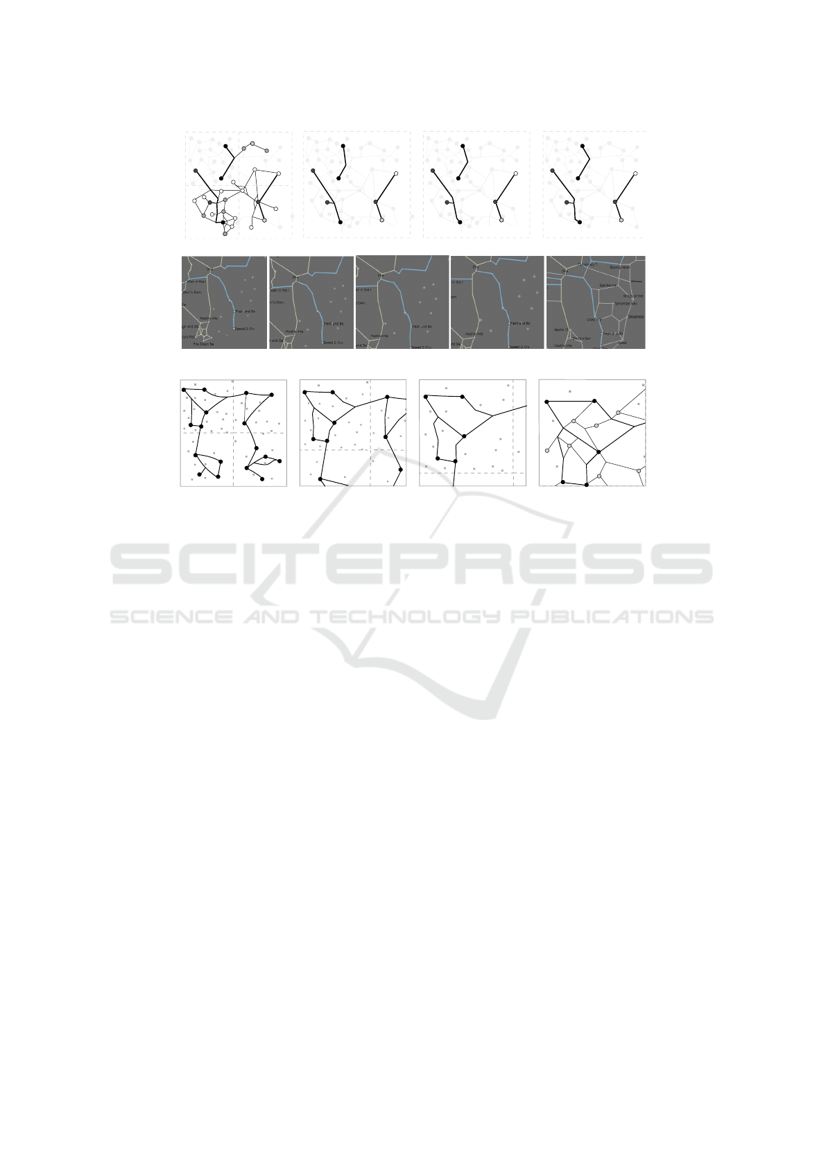
We draw the nodes as points, and edges as polyg-

onal chains. Each maximal straight line segment in

the drawing is called a rail. The edges may share

rails. Every point where a pair of rails meet is ei-

ther a node or a point which we call a junction. Fig-

ure 1(a) depicts a traditional node-link diagram of a

108

Mondal, D. and Nachmanson, L.

A New Approach to GraphMaps, a System Browsing Large Graphs as Interactive Maps.

DOI: 10.5220/0006618101080119

In Proceedings of the 13th International Joint Conference on Computer Vision, Imaging and Computer Graphics Theory and Applications (VISIGRAPP 2018) - Volume 3: IVAPP, pages

108-119

ISBN: 978-989-758-289-9

(a) (b) (d)

(c)

(e)

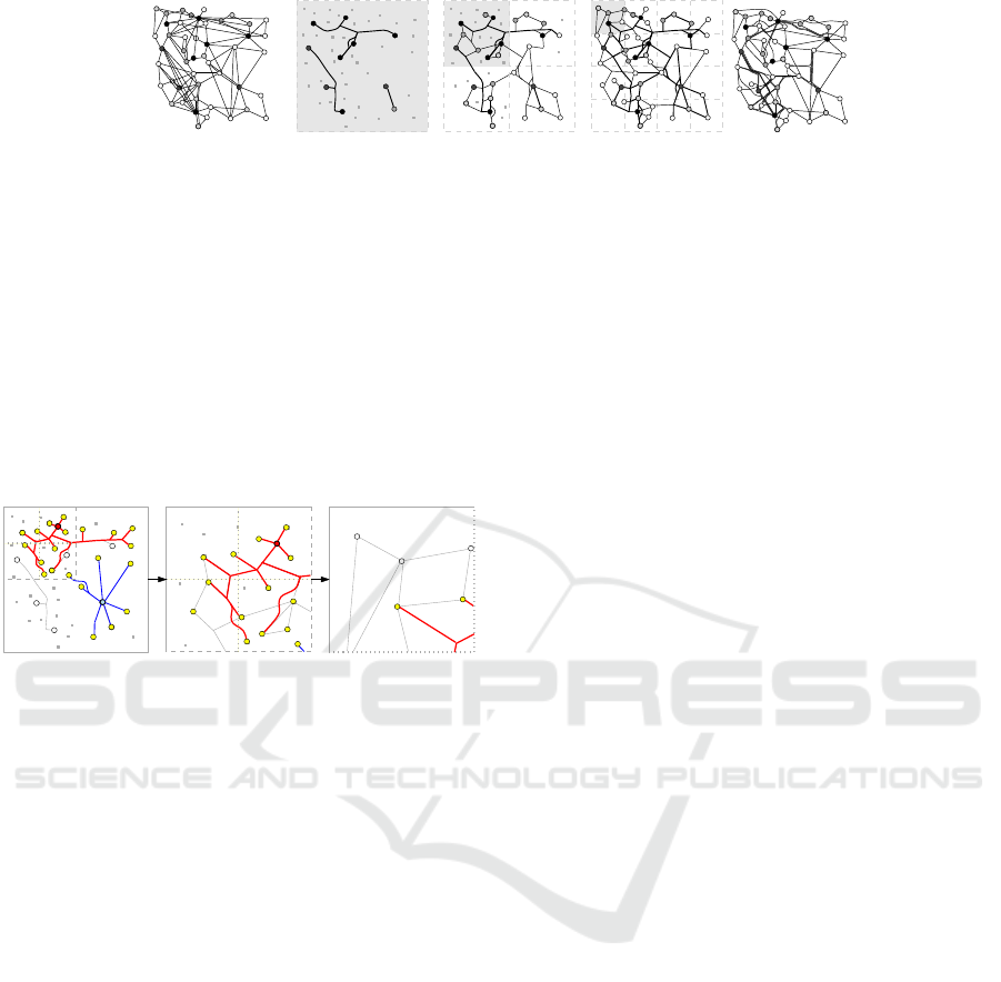
Figure 1: (a) A node-link diagram of a graph G. (b–d) A GraphMaps visualization of G. (e) An example of edge bundling.

graph G. Figures 1(b–c) illustrate a GraphMaps visu-

alization of G on three zoom levels. The gray region

at each level corresponds to a viewport in that level.

The higher ranked nodes of G have the darker color.

The tiny gray dots represent the locations of the nodes

that are not visible in the current layer. Figures 2 illus-

trate the node selection technique and the zoom fea-

ture. The rails rendered by thick lines correspond to

the shortest paths from the selected nodes a and h to

their neighbors.

Figure 2: Node selections and zoom in.

In our scheme, where we change the rendering de-

pending on the zoom level, the quality of the visu-

alization depends both on the quality of the drawing

on each level, and the differences between the draw-

ings of successive zoom levels. We think that a good

drawing of a graph on a single zoom level satisﬁes the

following properties:

- The angular resolution is large

- The degree at a node or at a junction is small.

- The amount of ink, that is the sum of the lengths

of all distinct rails used in the drawing, is small.

- The edge stretch factor or dilation, that is the ratio

of the length of an edge route to the Euclidean

distance between its end nodes, is small.

These properties help to follow the edge routes, re-

duce the visual load, and thus improve the readability

of a drawing. Since some of the principles contradict

each other, optimizing all of them simultaneously is a

difﬁcult task.

Our algorithm, in addition to creating a good

drawing of each G

, attempts to construct these draw-

ings in a way that a switch from G

to G

i+1

does not

cause a large change on the screen. We try to keep the

amount of new appearing details relatively small and

also try to keep the edge geometry stable.

1.1 Related Work

A large number of graph visualization tools, e.g.,

Centrifuge, Cytoscape, Gephi, Graphviz, Biolay-

out3d, have been developed over the past few decades

due to a growing interest in exploring network data.

A good visualization requires the careful placement

of nodes, e.g., sometimes nodes with similar proper-

ties are placed close to each other, whereas the nodes

that are dissimilar are placed far away. Force directed

approaches, multi-dimensional scaling and stochastic

neighbor embedding are some common techniques to

generate the node positions (Hu, 2005; Klimenta and

Brandes, 2012; van der Maaten and Hinton, 2008).

Techniques that try to make the visualization readable

by drawing the edges carefully consider various types

of edge bundling (Ersoy et al., 2011; Gansner et al.,

2011; Lambert et al., 2010; Pupyrev et al., 2011) and

edge routing techniques (Dobkin et al., 1997; Holten

and van Wijk, 2009; Dwyer and Nachmanson, 2009).

Informally, the edge bundling technique groups the

edges that are travelling towards a common direc-

tion, and routes these edges through some narrow

tunnel. Figure 1(e) illustrates an example of edge

bundling. Other forms of clutter reduction approaches

include node aggregation (Wattenberg, 2006; Dunne

and Shneiderman, 2013; Zinsmaier et al., 2012),

topology compression (Shi et al., 2013; Brunel et al.,

2014), and sampling algorithms (Gao et al., 2014).

This paper focuses on GraphMaps, proposed by

Nachmanson et al. (Nachmanson et al., 2015), that

reduces clutter by distributing nodes to different

zoom levels and routing edges on shared rails. Like

the clutter reduction approaches, a primary goal of

GraphMaps is to make the visualization more read-

able and interactive in the higher levels of abstrac-

tion. Nachmanson et al. (Nachmanson et al., 2015)

use multidimensional scaling to create the node posi-

tions. To distribute the nodes into zoom levels, they

consider at each level i, an uniform 2

×2

grid, where

each grid cell is called a tile. The tiles are ﬁlled with

nodes, the most important nodes ﬁrst. While ﬁlling

the levels with nodes, they maintain a node and a rail

quota that bound the number of nodes and rails inter-

secting a tile. Whenever an insertion of a new node

creates a tile intersecting more than one fourth of the

A New Approach to GraphMaps, a System Browsing Large Graphs as Interactive Maps

109

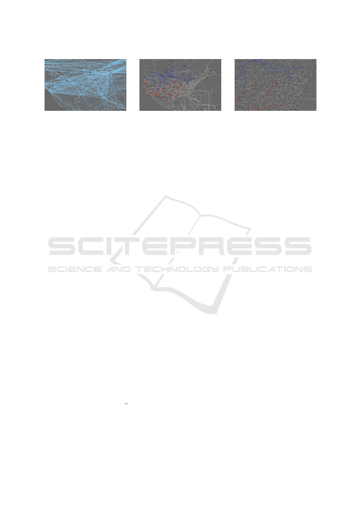
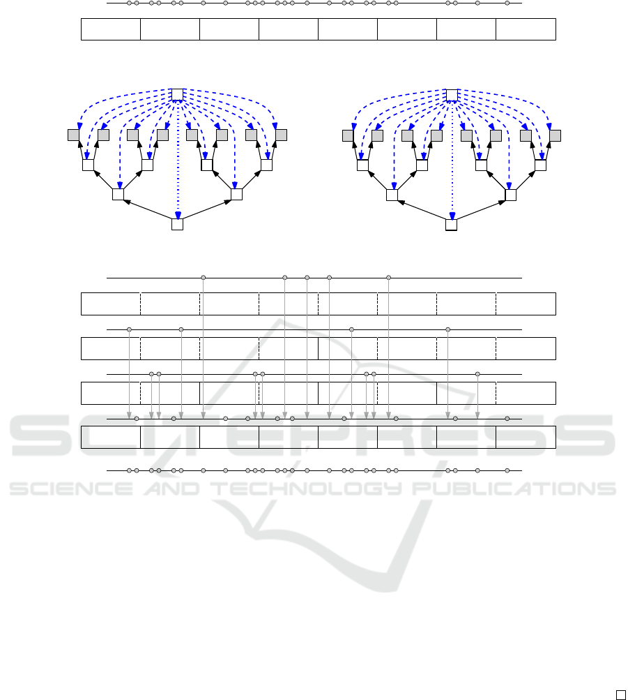
Figure 3: A partial display of a ﬂight network with approximately 3K nodes and 19K edges. (left) Traditional node-link

diagram over the airports of North America. (middle) The top-level of a GraphMaps visualization based on our approach,

where the airports TUS and YWG are selected. (right) A view after zoom in.

node quota nodes or more than one quarter of rail

quota rails, a new zoom level is created to insert the

rest of the entities. The visualization of GraphMaps

works in such a way that each viewport is covered

by four tiles of the current level. This ensures that

not more than the node quota nodes and the rail quota

rails are rendered per viewport.

GraphMaps visualization also relates to the hier-

archical visualization of clustered networks (Schaffer

et al., 1996; Balzer and Deussen, 2007). We refer the

reader to the survey (Vehlow et al., 2015) for more

details on visualizing graphs based on graph parti-

tioning. There exist some systems that render large

graphs on multiple layers by using the notion of tem-

poral graphs, e.g., evolving software systems (Coll-

berg et al., 2003; Lambert et al., 2010). A generaliza-

tion of stochastic neighbor embedding renders nodes

on multiple maps (van der Maaten and Hinton, 2012).

Gansner et al. (Gansner et al., 2010) proposed a visu-

alization that emphasizes node clusters as geographic

regions.

1.2 Contribution

The existing implementation of GraphMaps (Nach-

manson et al., 2015) focuses mainly on the quality of

the layout at individual zoom level. The construction

follows a top-down approach, where the successive

levels were obtained by inserting nodes incrementally

in a greedy manner.

We propose an algorithm to construct a

GraphMaps visualization starting from a com-

plete drawing of the graph G(= G

) at the bottom

level. Speciﬁcally, given an arbitrary mesh and the

edge routes of G

on this mesh, our method builds

the edge routes for G

k−1

,...,G

, in this order.

We introduce a particular type of mesh, called com-

petition mesh, which is of independent interest due to

its low edge stretch factor (2 +

√

2), and high angular

resolution 45

◦

. We then construct GraphMaps visual-

izations by applying our algorithm to this mesh. We

develop a node assignment algorithm that minimizes

the change in the drawing when switching from G

i+1

during zoom in, where 1 ≤i < k. Moreover, we

propose new node selection techniques to cope with

some of the challenges of the GraphMaps approach.

We also carried out experiments on some real-life

datasets (see Figure 3 and Section 5). Our experi-

ments reveal the usefulness of GraphMaps, even in its

basic implementations, for understanding the network

information through interactive exploration.

2 TECHNICAL BACKGROUND

We now introduce the mesh that we use for edge rout-

ing and analyze its properties. Let P be a set of n dis-

tinct points that correspond to the node positions, and

let R(P) be the smallest axis aligned rectangle that

encloses all the points of P. A competition mesh of

P is a geometric graph constructed by shooting from

each point, four axis-aligned rays at the same con-

stant speed (towards the top, bottom, left and right),

where each ray stops as soon as it hits any other ray

or R(P). We break the ties arbitrarily, i.e., if two non-

parallel rays hit each other simultaneously, then arbi-

trarily one of these rays stops and the other ray contin-

ues. If two rays are collinear and hit each other from

the opposite sides, then both rays stop. We denote

this graph by M(P), e.g., see Figure 4. The vertices

of M(P) are the points of P (nodes), and the points

where a pair of the rays meet (junctions). Two ver-

tices in M(P) are adjacent if and only if the straight

line segment connecting them belongs to M(P). A

competition mesh can also be viewed as a variation of

a motorcycle graph (Eppstein et al., 2008), or a ge-

ometric spanner with Steiner points (Bose and Smid,

2013). In the rest of the paper the term ‘vertices’ de-

notes all the nodes and junctions of M(P).

For any point u, let u

and u

be the x and y-

coordinates of u, respectively, and let l

(u) and l

(u)

be the vertical and horizontal straight lines through

u, respectively. For any two points p,q in R

, let

dist

(p,q) be the Euclidean distance between p and

q. For each point u of the plane we deﬁne four quad-

IVAPP 2018 - International Conference on Information Visualization Theory and Applications

110

(a) (b) (c) (d)

right

bottom

top

(t)

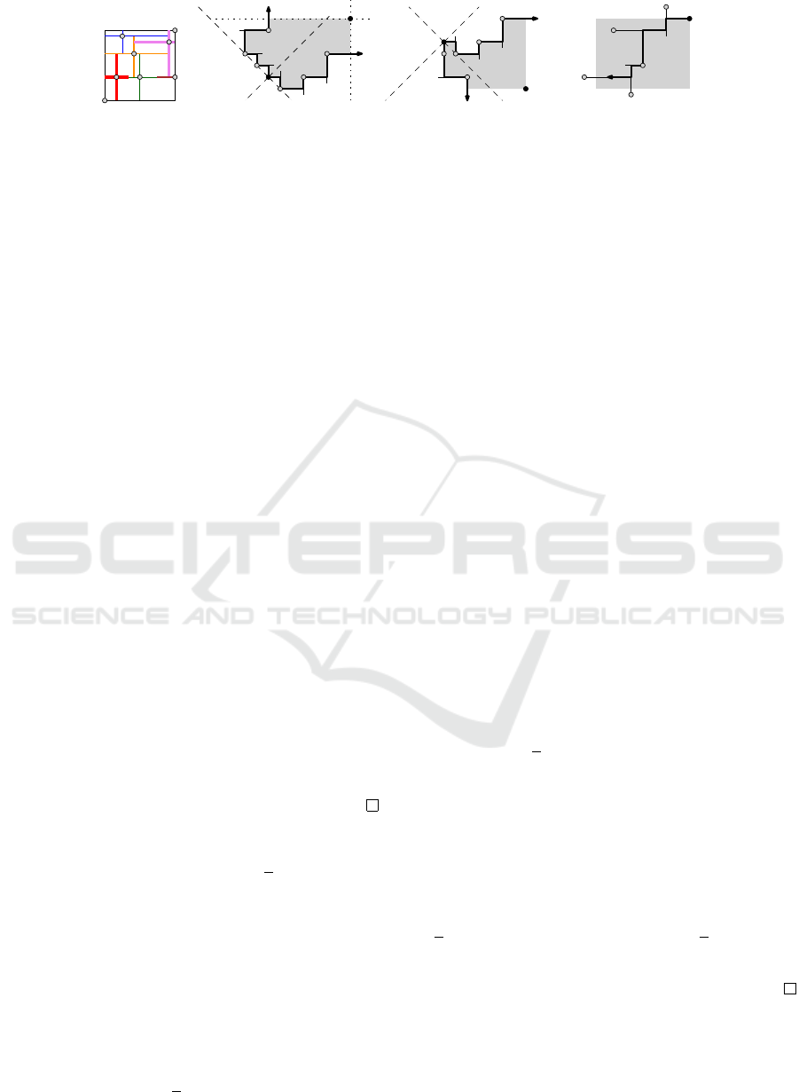
Figure 4: (a) A point set and its corresponding competition mesh. (b–c) Bounding the bottom-left quadrant of t. (d) A

monotone path inside the bottom-left quadrant of t.

rants formed by the horizontal and vertical lines pass-

ing through u. A path v

,...,v

is monotone in direc-

tion of vector a if for each 1 ≤ i < k the dot product

a·(v

i+1

−v

) is not negative. Lemmas 1–2 prove some

properties of M(P).

Lemma 1. Let u be a node in M(P). Then in each

quadrant of u there is a path in M(P) that starts at u,

ends at some point on R(P), and is monotone in both

horizontal and vertical directions.

Proof. Without loss of generality it sufﬁces to prove

the lemma for the ﬁrst quadrant of u, which consists of

the set of points v such that v

≥ u

and v

≥ u

. Sup-

pose for a contradiction that there is no such path in

this quadrant. Consider a maximal xy-monotone path

Π that starts at u and ends at some node or junction w

of M(P). If w is a node, then we extend Π using the

right or top ray of w, which is a contradiction. There-

fore, w must be a junction in M(P). Without loss of

generality assume that the straight line segment ` in-

cident to w is horizontal. Since Π is a maximal xy-

monotone path, the ray r

corresponding to ` must be

stopped by some vertical ray r

generated by some

vertex w

. Observe that w

> w

, otherwise we can

extend Π towards w

. Since r

is stopped, the ray r

must continue unless there are some other downward

ray r

that hits r

at w. In both cases we can extend

Π, either by following r

(if it continues), or follow-

ing the source of r

(if r

is stopped by r

), which

contradicts to the assumption that Π is maximal.

Lemma 2. For any set P with n points M(P) has O(n)

vertices and edges. The graph distance between any

two nodes of M(P) is at most (2 +

√

2) times the Eu-

clidean distance.

Proof. By construction of M(P), whenever a junction

is created, one ray stops. Since |P| = n there are at

most 4n rails, and therefore we cannot have more than

4n junctions, that proves that the number of vertices in

M(P) is O(n). Since M is a planar graph, the number

of edges is also O(n).

We now show that the ratio of the graph distance

and the Euclidean distance between any two nodes of

M(P) is at most (2 +

√

2). Let C

le f t

right

top

, and

bottom

be the four cones with the apex at (0,0) deter-

mined by the lines y = ±x. Let s and t be two nodes

in M(P). Without loss of generality assume that s lo-

cated at (0,0) and t lies on C

right

. Consider now an x-

monotone orthogonal path P

right

= (v

,...,v

)

in the mesh such that v

coincides with s, for each

0 < i ≤ q, v

is a node in M(P) that stops the right-

ward ray of v

i−1

, and v

lies on or to the right of l

(t),

e.g., see Figure 4(b). Suppose that t is either above

or below P

right

. If t is above P

right

, then consider a y-

monotone path P

top

= (w

, w

,...,w

) such that

coincides with s, for each 0 < i ≤ r, w

is a node in

M(P) that stops the upward ray of v

i−1

, and v

lies on

or above l

(t). If t is below P

right

, then deﬁne a path

bottom

symmetrically, e.g., see Figure 4(c).

Without loss of generality assume that t is above

right

. Observe that the paths P

top

and P

right

remain

inside the cones C

top

and C

right

, respectively, and

bound the bottom-left quadrant of t, as shown in the

shaded region in Figure 4(b). By Lemma 1, t has a

(−x)(−y)-monotone path P that starts at t and reaches

the boundary of R(P), e.g., see Figure 4(d). This

path P must intersect either P

top

or P

right

. Hence

we can ﬁnd a path P

from s to t, where P

starts

at s, travels along either P

top

or P

right

depending on

which one P intersects, and then follows P from the

intersection point. We now show that length of P

at most (2 +

√

2) ·dist

(s,t). Since any ray is not

shorter than a ray it stops, the sum of the lengths

of the vertical segments of P

right

is at most the sum

of the lengths of the horizontal segments. Therefore,

the part of P

right

inside the bottom-left quadrant of t

is at most 2t

. Similarly, the part of P

top

inside the

bottom-left quadrant of t is at most 2t

. Path P is

not longer than t

+ t

(see Figure 4(d)) . Therefore,

the length of P

is at most t

+ t

+ 2 ·max{t

)} ≤

√

2·dist

(s,t)+2·max{t

}≤(2+

√

2)·dist

(s,t).

In the case when t belongs to P

right

, the length of

path P is zero and the proof easily follows.

The following lemma states that a competition

mesh can be constructed in O(nlogn) time.

Lemma 3. For any set P with n points, the competi-

tion mesh M(P) can be constructed in O(nlogn) time.

A New Approach to GraphMaps, a System Browsing Large Graphs as Interactive Maps

111

Proof. Deﬁne for each point w ∈P, a set of eight non-

overlapping cones as follows: The central angle of

each cone is 45

◦

and the cones are ordered counter

clockwise around w. The ﬁrst cone lies in the ﬁrst

quadrant of w between the lines y = x +w

and y = 0,

as shown in Figure 5(a). Guibas and Stolﬁ (Guibas

and Stolﬁ, 1983) showed that in O(n log n) time, one

can ﬁnd for every point w ∈ P the nearest neigh-

bor of w (according to the Manhattan Metric) in

each of the eight cones of w. Assume that δ

{min

{a,b}∈P, where a

6=b

−b

|}, which can be com-

puted in O(n log n) time by sorting the points accord-

ing to y-coordinates.

We construct M in four phases. The ﬁrst phase

iterates through the top rays of the each point w and

ﬁnds the point w

closest to l(h)

(in Manhattan met-

ric) such that |w

−w

| ≤ |w

−w

|. Note that if such

a w

exists, then one of the horizontal rays r

of w

would reach the point (w

) before the top ray r of

w (while all rays are grown in an uniform speed). Ac-

cording to the deﬁnition of the competition mesh, we

can continue the ray r

and stop growing the ray r. If

no such w

exists, then r must hit R(P).

To ﬁnd the point w

, it sufﬁces to compare the

Manhattan distances of the nearest neighbors in the

second and third cones of w (breaking ties arbitrar-

ily). Since the nearest neighbors at each cone can

be accessed in O(1) time, we can process all the top

rays in linear time. Figure 5(b) shows the junctions

and nodes created after the ﬁrst phase, where all the

rays that stopped growing are shown in thin lines.

The nearest neighbors in the second and third cones

of w are a and b, respectively. Since a is closer to

(w) than b, the top ray of w does not grow beyond

). The second phase processes the bottom rays

in a similar fashion, e.g., see Figure 5(c). Both the

ﬁrst and second phase use a ray shooting data struc-

ture to check whether the current ray already hits an

existing ray. We describe this data structure in the

next paragraph while discussing phase three. Let the

planar subdivision at the end of phase two be S.

In the third phase, we grow each left ray until it

hits any other vertical segment in S, as follows: For

each vertical edge ab in S, construct a segment a

shrinking ab by δ

/3 from both ends. For each node

and junction w, construct a segment w

such that

= (w

−δ

/4) and w

= (w

+δ

/4). Let S

be the constructed segments. Note that the segments

in S

are non-intersecting. Giyora and Kaplan (Giy-

ora and Kaplan, 2009) gave a ray shooting data struc-

ture D that can process O(n) non-intersecting verti-

cal rays in O(n log n) time, and given a query point

q, D can ﬁnd in O(log n) time the segment (if any) in

immediately to the left of q. Furthermore, D sup-

ports insertion and deletion in O(log n) time. For each

point q ∈ P in the increasing order of x-coordinates,

we shoot a leftward ray r from q, and ﬁnd the ﬁrst

segment ab hit by the ray. Assume that a

< b

and r

hits ab at point x. We update the subdivision S accord-

ingly, then delete segment ab from D, and insert seg-

ment xb in D. Note that these updates keep all the seg-

ments in D non-intersecting. Since there are O(n) left

rays, processing all these rays takes O(n log n) time.

Figure 5(d) illustrates the third phase.

The fourth phase processes the right rays in a

similar fashion, e.g., see Figure 5(e). Since the

preprocessing time of the data structures we use is

O(nlogn), and since each phase runs in O(nlogn)

time, the construction of the computation mesh takes

O(nlogn) time in total.

3 GRAPHMAPS SYSTEM

Our technique for calculating the graphs G

,...,G

(equivalently, node level assignment) is described in

Section 4. For now, let us assume that the sequence

of graphs is ready. We now show how to route edges

on graphs G

The computation of edges starts from the bottom.

Namely we build a competition mesh M for graph

G(= G

). We route each edge (u, v) ∈ G as a short-

est path P

in M. Let us denote by M

the mesh we

obtain after applying these modiﬁcations to M. Next

we modify M

to make the routes more visually ap-

pealing. We perform local modiﬁcations and try to

minimize the total ink of the routes, which is the sum

of lengths of edges of M

used in the routes (Gansner

and Koren, 2006), and remove thin faces. During the

modiﬁcations we keep the angular resolution greater

or equal than some α > 0, and the minimum distance

between non-incident vertices and edges of M

greater

or equal than some β > 0. The local modiﬁcations are

described below.

Face reﬁnement: For each face f of M

that does

not contain a node of G in its boundary, we compute

the width of f , which is the smallest Euclidean dis-

tance between any two non-adjacent rails of f . If

the width of f is smaller than some given threshold,

then remove the longest edge of f from M

(breaking

ties arbitrarily). Figures 6(a–b) depict such a removal,

where the thin face is shown in gray. The edge routes

using the removed edge are rerouted through the re-

maining boundary of f

Median: Move each junction κ of M

toward the

geometric median of its neighbors, i.e., the point that

minimizes the sum of distance to the neighbors, as

long as the restriction mentioned above holds. Iterate

IVAPP 2018 - International Conference on Information Visualization Theory and Applications

112

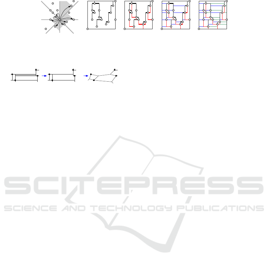
(a) (b) (c) (d) (e)

Figure 5: (a) A point set P and the nearest neighbor of w in each of the eight cones around w. (b–e) Construction of the mesh

of P, while processing (b) top rays, (c) bottom rays, (d) left rays and (e) right rays.

(a)

(b)

(c)

Figure 6: (a–b) Removal of thin faces. (b–c) Moving junc-

tions towards median.

the move for a certain number of times, or until the

change becomes smaller than some given threshold.

Figures 6(c–d) illustrate the outcome of this step.

Shortcut: Remove every degree two junction and

replace the two edges adjacent to it by the edge short-

cutting the removed junction, as long as the restriction

mentioned above holds.

In all the above modiﬁcations, the routes are

updated accordingly. Modiﬁcations “Median” and

“Shortcut” diminish the ink. The ﬁnal M

gives the

geometry of the bottom-level drawing of G in our ver-

sion of GraphMaps.

Given a mesh M

representing the geometry for

the drawing of G

, where 1 < i ≤ k, we construct

i−1

from M

by removing from the latter the nodes

V (G

) \V (G

i−1

), and by removing the edges that are

not used by any route P

u,v

, where (u,v) is an edge

of G

i−1

. Some routes P

u,v

can be straightened in

i−1

. We use the simpliﬁcation algorithm (Douglas

and Peucker, 1973) to morph the paths of M

to paths

of M

i−1

. Figures 7(a–b) illustrate the simpliﬁcation.

This change in the edge routes geometry dimin-

ishes the consistency between the drawings of succes-

sive levels. To smoothen the differences while transit-

ing from zoom level i to i + 1 we linearly interpolate

between the paths of M

and M

i+1

, as demonstrated in

Figures 7(b–d).

The idea of path simpliﬁcation and transition

via linear interpolation enables us to construct

GraphMaps in a bottom-up approach. In fact, the

above strategy can be applied to transform any mesh

generated from a set of 2D points to a GraphMaps vi-

sualization.

4 COMPUTING NODE LEVELS

Let us consider in more details how the view changes

when we zoom by examining Figures 8(a)–(d). On

the top-left tile of Figure 8(a), the user’s viewport cov-

ers the whole graph, so G

is exposed. In Figure 8(d),

the user’s viewport contains only the top-left tile of

Figure 8(a), and the visualization switches to graph

. Seven new nodes, which were not fully visible

in zoom level 1, become fully visible for the current

viewport, as represented in light gray. If all of a sud-

den, a large number of new nodes become fully visi-

ble, then it may disrupt user’s mental map. Here we

propose an algorithm to keep this change small.

We build the tiles as in (Nachmanson et al., 2015).

In the ﬁrst level we have only one tile coinciding

with the graph bounding box. On the ith level, where

i > 1, the tiles are obtained by splitting each tile in the

(i −1)th level into a uniform 2 ×2 grid cell. This ar-

rangement of tiles can be considered as a rooted tree

T , where the tiles correspond to the nodes of the tree.

Speciﬁcally, the topmost tile is the root of T , and a

node u is a child of another node v if the correspond-

ing tiles t

and t

lie in two different but adjacent lev-

els, and t

⊂t

. We refer to T as a tile tree.

For every node v in T , denote by S(v) the num-

ber of fully visible nodes in the tile t

. For an edge

e = (v, w) in T , where v is a parent of w, we denote by

the number of new nodes that become visible while

navigating from t

to t

, i.e., δ

= |S(w) \S(v)|. We

can control the rate the nodes appear and disappear

from the viewport by minimizing

∑

e∈E(T )

, where

E(T ) is the set of edges in T . For simplicity we show

how to solve the problem in one dimension, where all

the points are lying on a horizontal line. It is straight-

forward to extend the technique in R

Problem. BALANCED VISUALIZATION

Input. A set P of n points on a horizontal line,

where every point q ∈ P is assigned a rank r(q).

A tile tree T of height ρ; and a node quota Q, i.e.,

the number of points allowed to appear in each

tile.

Output. Compute a mapping g : P → {1,2,...ρ}

A New Approach to GraphMaps, a System Browsing Large Graphs as Interactive Maps

113

(a) (b) (c) (d)

Figure 7: (a) Zoom level 2. (b–d) Transition from level 1 to 2. (bottom) Transition in our GraphMaps system.

(a)

(b)

(c)

(d)

Figure 8: (a) Zoom level 1. (b–c) Transition from level 1 to 2. (d) Zoom level 2.

(if exists) that

- satisﬁes the node quota,

- minimizes the objective F =

∑

e∈E(T )

, and

- for every pair of points q,q

∈ P with r(q) ≥

r(q

), satisﬁes the inequality g(q) ≤ g(q

which we refer to as the rank condition.

If the rank of all the points are distinct, then the

solution to BALANCED VISUALIZATION is unique,

and can be computed in a greedy approach. But the

problem becomes non-trivial when many points may

have the same rank. In this scenario, we prove that the

BALANCED VISUALIZATION problem can be solved

in O(τ

log

τ) + O(nlogn) time, where τ is the num-

ber of nodes in T . This is quite fast since the maxi-

mum zoom level is a small number, i.e., at most 10,

in practice. We reduce the problem to the problem of

computing a minimum cost maximum ﬂow problem,

where the edge costs can be convex (Orlin, 1993; Or-

lin and Vaidyanathan, 2013), e.g., quadratic function

of the ﬂow passing through the edge. Figure 9(a) de-

picts a set of points on a line, where the associated

tiles are shown using rectangular regions. The num-

bers in each rectangle is the number of points in the

corresponding tile. Figure 9(b) shows a correspond-

ing network G, where the source is denoted by s, and

the sinks are denoted by T

,...,T

. The excess at

the source and the deﬁcit at the sinks are written in

their associated squares. We allow each internal node

w (unﬁlled square) of the tile tree to pass at most Q

units of ﬂow through it. This can be modeled by re-

placing w by an edge (u,v) of capacity Q, where all

the edges incoming to w are incident to u and the out-

going edges are incident to v. This transformation is

not shown in the ﬁgure. Set the capacity of all other

edges to ∞.

The production of the source is n units, and the

units of ﬂow that each sink can consume is equal to

the number of points lying in the corresponding tile.

The cost of sending ﬂows along the tree edges (solid

black) is zero. The cost of sending ﬂows along the

dotted edge connecting the source and the tree root is

also zero. The cost of sending x units of ﬂow along

the dashed edges is x

; sending x units of ﬂow through

a dashed edge corresponds to x new nodes that are be-

coming visible when we zoom in at the tile of the edge

target. Figure 9(c) illustrates a solution to the mini-

mum cost maximum ﬂow problem, where the ﬂows

are interpreted as follows:

(A) The number in a square denotes the number of

points that would be visible in the associated tile.

(B) The edges (s,w), where w is not the root, are la-

beled by numbers. Each such number corresponds

to the new nodes that will appear while zooming

in from the tile associated to parent(w) to the tile

associated to w. Thus the cost of this network ﬂow

is the sum of the squares of these numbers, i.e., 35.

IVAPP 2018 - International Conference on Information Visualization Theory and Applications

114

2 4 4 5 5 2 3 1

2 4

5 2

3 1

2 4 4 5 5 2 3 1

(a)

(b) (c)

(d)

root

Figure 9: (a) A set of points on a line and the associated tiles are shown using rectangular regions. (b) A corresponding

network G. (c) A solution to the minimum cost maximum ﬂow problem. (d) A solution to the BALANCED VISUALIZATION

problem that corresponds to the network ﬂow.

of nodes that are fully visible both u and in v.

(D) Any one unit source-to-sink ﬂow corresponds

to a point of P, where the ﬂow path source,

,...,u

(= sink) denotes that the point ap-

peared in all the tiles associated to u

,...,u

Lemma 4. A minimum cost maximum ﬂow in G mini-

mizes the objective function F of the BALANCED VI-

SUALIZATION problem.

Proof. If the amount of ﬂow consumed at sink is

smaller than n, then we can ﬁnd a cut in G with to-

tal capacity less than n. Thus even if we saturate the

corresponding tiles with points from P, we will not be

able to visualize all the points without violating the

node quota. Therefore, we can visualize all the points

if and only if the ﬂow is maximum and the total con-

sumption is n. Therefore, the only concern is whether

the solution with cost λ obtained from ﬂow-network

model minimizes the sum of the squared node differ-

ences between every parent and child tiles. Suppose

for a contradiction that there exists another solution

of BALANCED VISUALIZATION with cost λ

< λ. In

this scenario we can label the edges of the network

according to the interpretation used in (A)–(D) to ob-

tain a maximum ﬂow in G with cost λ

. Therefore, the

minimum cost computed via the ﬂow-network model

cannot be λ, a contradiction.

Given a solution to the network ﬂow, we can con-

struct a corresponding solution to the BALANCED VI-

SUALIZATION problem as described below.

- For each point w, set g(w) = ∞.

- For each zoom level z from ρ to 1, process the tiles

of zoom level z as follows. Let W be a tile in zoom

level z. Find the amount of ﬂow x incoming to W

from s in G. Note that this amount x corresponds

to the difference in the number of points between

A New Approach to GraphMaps, a System Browsing Large Graphs as Interactive Maps

115

W and parent(W ). Therefore, we ﬁnd a set L of x

lowest priority points in W with zoom level equal

to ∞, then for each w ∈ L, we set g(w) = z. Fig-

ure 9(d) illustrates a solution to the BALANCED

VISUALIZATION problem that corresponds to the

network ﬂow of Figure 9(c).

If the resulting mapping does not satisfy the rank con-

dition, then the instance of BALANCED VISUALIZA-

TION does not have any afﬁrmative solution. The

best known running time for solving a convex cost

network ﬂow problem on a network of size O(τ) is

O(τ

log

τ) (Orlin, 1993; Orlin and Vaidyanathan,

2013). Besides, it is straightforward to compute the

corresponding node assignments in O(nlogn) time

augmenting the merge sort technique with basic data

structures. Hence we obtain the following theorem.

Theorem 1. Given a set of n points in R, a tile tree of

τ nodes, and a quota Q, one can ﬁnd a balanced visu-

alization (if exists) in O(τ

log

τ)+O(nlogn) time.

While implementing GraphMaps, we need to

choose a node quota Q depending on the given total

number of zoom levels ρ. Using a binary search on

the number of nodes, in O(logn) iterations, one can

ﬁnd a minimal node quota that allow visualizing all

the points of P satisfying the rank condition.

5 EXPERIMENTS

The GraphMaps system proposed previously (Nach-

manson et al., 2015) uses

to obtain the graph for

routing edges on a level. Our approach does not de-

pend on Triangle, but uses Competition Mesh. This

has several advantages. For example, Competition

Mesh usually produces less edges than Triangle. As

a result the edge routing runs much faster. With the

same initial layout for the nodes, the GraphMaps sys-

tem based on our approach sped up the initial pro-

cessing signiﬁcantly, up to 8 times on some graphs.

The graph with 38395 nodes and 85763 edges was

processed in the new system within 1 hour and 45

minutes, where the previous GraphMaps system took

6 hours (Nachmanson et al., 2015). Besides, Com-

petition Mesh is more robust than Triangle. We did

not experience failures, which were reported on Tri-

angle (Nachmanson et al., 2015).

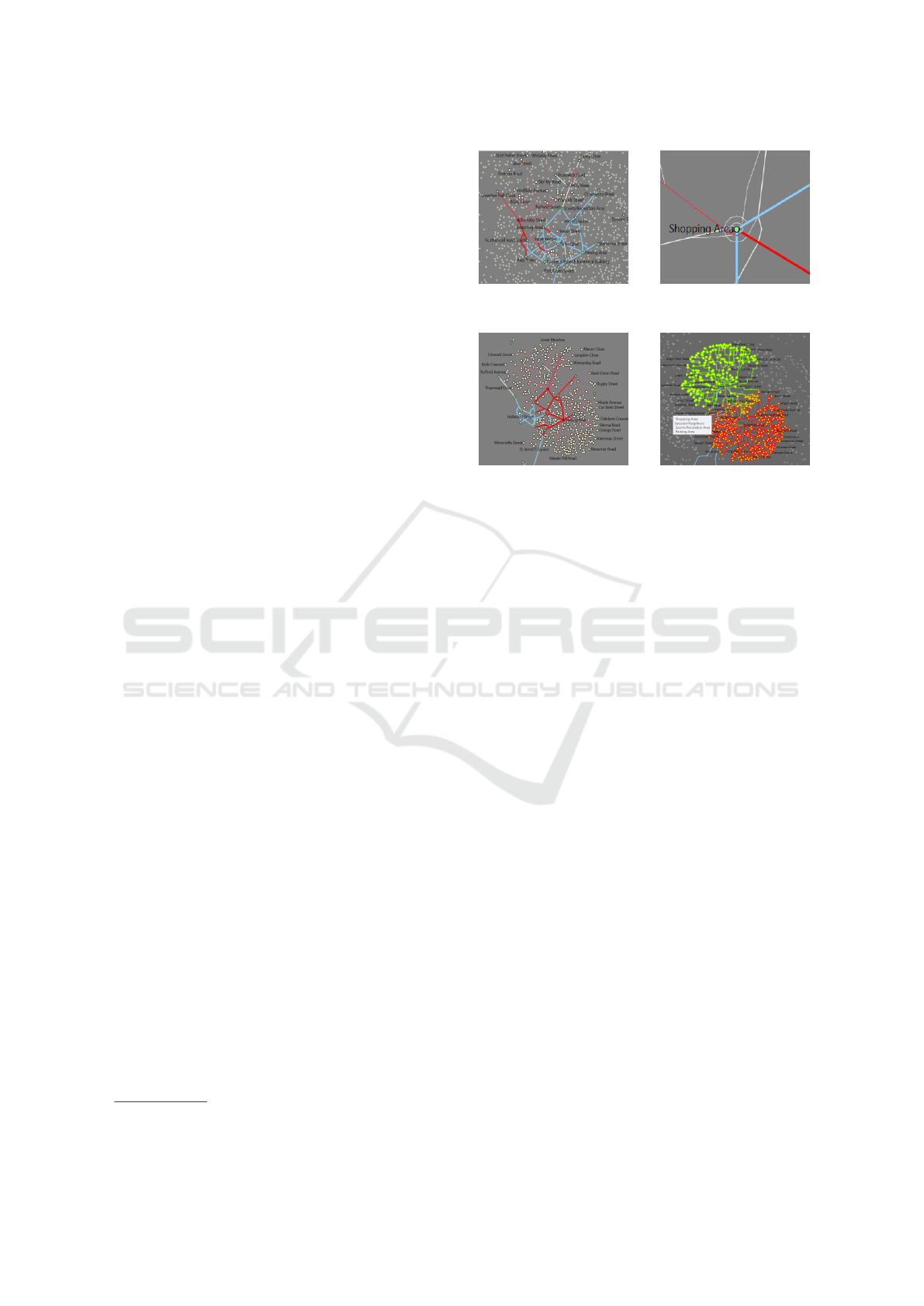
The previous GraphMaps (Nachmanson et al.,

2015) supports node selection, which is initiated by

the user clicks. Selection of a node highlights the

paths to its neighbors in red. This may create am-

biguity. For example, Figure 10(top-left) shows a

https://www.cs.cmu.edu/

∼

quake/triangle.html

Figure 10: Node selection in previous GraphMaps (Nach-

manson et al., 2015).

Figure 11: Selection of multiple nodes: (a) previous

GraphMaps (Nachmanson et al., 2015), and (b) our ap-

proach.

graph of Burglary events (April 2015) in Manchester,

UK, where two events are adjacent if they are lo-

cated within 1km of each other. Selection of the node

‘Burnaby Street’ highlights a rail very close to the

node ‘Shopping area’, which gives a false impres-

sion that these nodes are adjacent. After zooming

in one can see that there is a detour that carries the

highlighted path away from ‘Shopping area’, e.g., see

Figure 10(top-right). This also give a wrong impres-

sion of the node degree. Besides, since the edges may

share rails, selection of multiple nodes may obscure

the adjacency relationship, e.g., see Figure 11(left).

We introduce new visualizations that allow the

user to better understand the node neighborhood.

Clicking on a node toggles its status from selected to

not selected. When a node is selected, its neighbors

are highlighted in yellow color, and the edges con-

necting the clicked node with the neighbors are high-

lighted with some unique color. If the mouse pointer

hovers over a node highlighted by yellow color, then

a tooltip appears with the list of the node neighbors,

e.g., see Figure 11(right). When a selected node is

unselected, then every edge adjacent to it is rendered

in the default color, and the highlighting is removed

from each neighbor, unless it is a neighbor of another

selected node. These visualization measures help to

resolve some ambiguities caused by edge bundling.

Note that our approach does not create any detour,

and thus avoids the circular artifacts (rails) around the

nodes. Exploring the node adjacencies and degree be-

comes comparatively easy, and less number of rails

aids faster level transition.

Like the previous GraphMaps, our approach can

IVAPP 2018 - International Conference on Information Visualization Theory and Applications

116

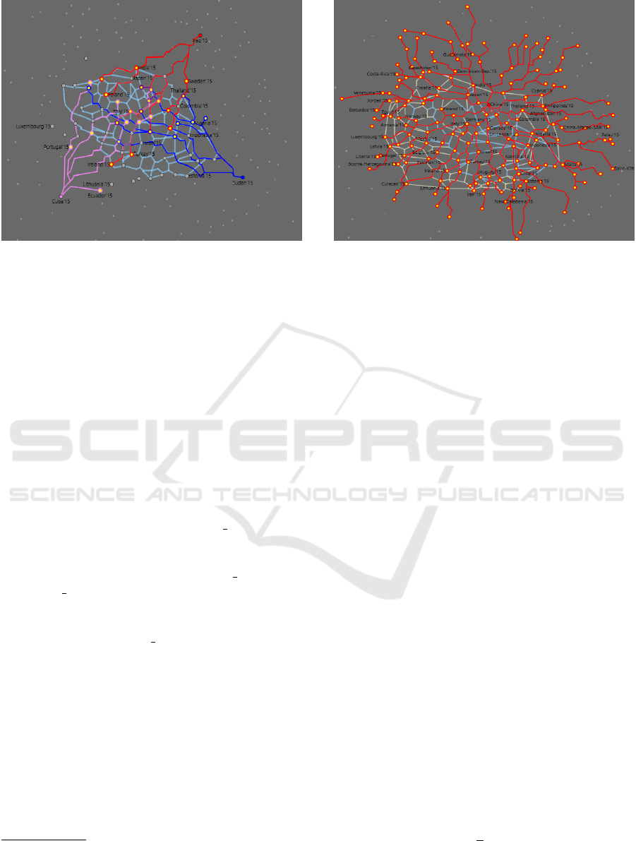
Figure 12: A visualization of gemstone trade-relation among countries (≈7K edges) in 2015 (https://resourcetrade.earth).

Selected nodes: (left) Iraq, Sudan, Cuba, and (right) China.

also revel the structural properties of the graph. Fig-

ure 12 depicts a gemstone trade graph, where the

countries with most trade relation, e.g., China, are

in the central position and the countries with small

number of trade relations fall into the periphery. Fig-

ure 13 visualizes a drugs-crime event in Manchester,

UK, where the events are connected if they are lo-

cated within a distance of (left) 1Km and (right) 5Km

of each other. The high risk events form clusters in

the top-level visualizations.

Figure 14 shows an experiment with the graph of

include dependencies of the C++ sources of

. The de-

veloper was interested in how his ﬁles are used by the

rest of the system. He clicked node ‘lar solver.h’ rep-

resenting an important header ﬁle of his ﬁles and cre-

ated the neighborhood in red color (the upper draw-

ing). Then he noticed that ﬁle ‘theory lra.cpp’ in-

cludes ‘lar solver.h’ and clicked the former, creating

the blue neighborhood (in the lower drawing). Then

he noticed two ﬁles, marked by the black oval, that

were included into ‘theory lra.cpp’ by mistake.

In another experiment, a user was analyzing col-

laboration between Chinese and Russian composers

in 20-th and 21-st centuries. By highlighting the

neighborhoods of Chinese composers of 20-th cen-

tury, the user saw that there were no connections be-

tween the composers of these two countries in this

period. In 21-st century the only relation of such

kind that he found was between Tan Dun and Soﬁa

Gubaidulina. More details can be seen in a video

https://github.com/Z3Prover/z3

https://www.youtube.com/watch?v=qCUP20dQqBo&

feature=youtu.be

6 LIMITATIONS

Adjacency relations and node degrees are readily

visible in small size traditional node-link diagrams,

GraphMaps can process large networks, but it looses

those two aspects at an expense of avoiding clutter.

The users need to select nodes to explore the adjacen-

cies and node degrees. Currently, we use colors to

disambiguate node selections, which limits us to the

selection of a small number of nodes avoiding ambi-

guity. GraphMaps is sensitive to node quota or the

maximum number of nodes per tile. Selecting a large

node quota may increase the interaction latency dur-

ing level transitions. On the other hand, selecting a

small node quota may select few nodes on the top-

level, which may fail to give an overview of the graph

structure. An appropriate choice of the node quota

based on the graph size and node layout is yet to dis-

cover. For simplicity, we used polygonal chains to

represent the edges, different colors for multiple node

selections, and color transparency to avoid ambiguity.

It would be interesting to ﬁnd ways of improving the

visual appeal of a GraphMaps visualization, e.g., us-

ing splines for edges, enabling tooltip texts for show-

ing quick information and so on.

7 CONCLUSION

We described our algorithm to construct GraphMaps

Visualizations using competition mesh. Recall that

the edge stretch factor of the competition mesh we

created is at most (2 +

√

2). A natural open question

is to establish tight bound on the edge stretch factor of

the competition mesh. It would also be interesting to

A New Approach to GraphMaps, a System Browsing Large Graphs as Interactive Maps

117

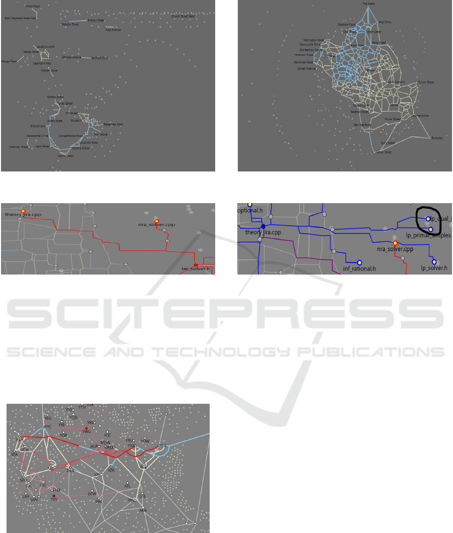
Figure 13: A visualization of drugs-crime event in Manchester, UK, with approximately (left) 0.5K edges, and (right) 8K

edges. The rails in light blue and white illustrate the ﬁrst and second zoom levels, respectively.

Figure 14: Highlighting the neighborhood in a unique color helps to understand relations.

ﬁnd bounded degree spanners (possibly with Steiner

points) that are monotone and have low stretch fac-

tor. We refer the reader to (Bose and Smid, 2013;

Dehkordi et al., 2015; Felsner et al., 2016) for more

details on such geometric mesh and spanners. We

leave it as a future work to examine how the quality

of a GraphMaps system may vary depending on the

choice of geometric mesh.

Figure 15: A visualization of the ﬂight network

dataset (https://openﬂights.org/data.html) using previous

GraphMaps (Nachmanson et al., 2015).

The previous GraphMaps (Nachmanson et al.,

2015) uses an incremental mesh generation, which

does not require path simpliﬁcation. Since the con-

struction of the upper levels does not take the lower

level nodes into account, the top-level view is usually

sparse, e.g., see Figure 15. Our approach is powerful

in the sense that any mesh can be transformed into a

GraphMaps visualization. But the upper levels are the

simpliﬁcation of the bottom level mesh, and thus the

quality of the top-level depends on both the bottom

level mesh and the simpliﬁcation process. It will be

interesting to further explore the pros and cons of both

approaches. We believe that our results will inspire

further research to enhance the appeal and usability

of GraphMaps visualizations.

ACKNOWLEDGEMENTS

This work was initiated when the ﬁrst author was

a summer intern at Microsoft Research, Redmond,

USA. His subsequent work was partially supported

by NSERC.

REFERENCES

Balzer, M. and Deussen, O. (2007). Level-of-detail vi-

sualization of clustered graph layouts. In Asia-

Paciﬁc Symp. on Visualization (APVIS), pages 133–

140. IEEE Computer Society.

Bose, P. and Smid, M. H. M. (2013). On plane geometric

spanners: A survey and open problems. Computa-

tional Geometry, 46(7):818–830.

IVAPP 2018 - International Conference on Information Visualization Theory and Applications

118

Brin, S. and Page, L. (2012). Reprint of: The anatomy of a

large-scale hypertextual web search engine. Computer

Networks, 56(18):3825–3833.

Brunel, E., Gemsa, A., Krug, M., Rutter, I., and Wagner,

D. (2014). Generalizing geometric graphs. J. Graph

Algorithms Appl., 18(1):35–76.

Collberg, C. S., Kobourov, S. G., Nagra, J., Pitts, J., and

Wampler, K. (2003). A system for graph-based visu-

alization of the evolution of software. In ACM Symp.

on Software Visualization (SOFTVIS), pages 77–86.

ACM.

Dehkordi, H. R., Frati, F., and Gudmundsson, J. (2015).

Increasing-chord graphs on point sets. J. Graph Al-

gorithms Appl., 19(2):761–778.

Dobkin, D. P., Gansner, E. R., Koutsoﬁos, E., and North,

S. C. (1997). Implementing a general-purpose edge

router. In Graph Drawing (GD), volume 1353 of

LNCS, pages 262–271. Springer.

Douglas, D. and Peucker, T. (1973). Algorithms for the re-

duction of the number of points required to represent

a digitized line or its caricature. The Canadian Car-

tographer, 10(2):112–122.

Dunne, C. and Shneiderman, B. (2013). Motif simpliﬁca-

tion: improving network visualization readability with

fan, connector, and clique glyphs. In ACM SIGCHI

Conference on Human Factors in Computing Systems

(CHI), pages 3247–3256. ACM.

Dwyer, T. and Nachmanson, L. (2009). Fast edge-routing

for large graphs. In Graph Drawing (GD), volume

5849 of LNCS, pages 147–158. Springer.

Eppstein, D., Goodrich, M. T., Kim, E., and Tamstorf, R.

(2008). Motorcycle graphs: Canonical quad mesh par-

titioning. Comput. Graph. Forum, 27(5):1477–1486.

Ersoy, O., Hurter, C., Paulovich, F. V., Cantareiro, G., and

Telea, A. (2011). Skeleton-based edge bundling for

graph visualization. IEEE Trans. Vis. Comput. Graph.,

17(12):2364–2373.

Felsner, S., Igamberdiev, A., Kindermann, P., Klemz, B.,

Mchedlidze, T., and Scheucher, M. (2016). Strongly

monotone drawings of planar graphs. In Symposium

on Computational Geometry, volume 51 of LIPIcs,

pages 37:1–37:15.

Gansner, E. R., Hu, Y., and Kobourov, S. G. (2010). Gmap:

Visualizing graphs and clusters as maps. In IEEE Pa-

ciﬁc Visualization Symp. (PaciﬁcVis), pages 201–208.

Gansner, E. R., Hu, Y., North, S. C., and Scheidegger, C. E.

(2011). Multilevel agglomerative edge bundling for

visualizing large graphs. In IEEE Paciﬁc Visualization

Symp. (PaciﬁcVis), pages 187–194.

Gansner, E. R. and Koren, Y. (2006). Improved circular

layouts. In Graph Drawing, LNCS, pages 386–398.

Springer.

Gao, R., Hu, P., and Lau, W. C. (2014). Graph property

preservation under community-based sampling. In

IEEE Global Communications Conference (GLOBE-

COM), pages 1–7.

Giyora, Y. and Kaplan, H. (2009). Optimal dynamic vertical

ray shooting in rectilinear planar subdivisions. ACM

Transactions on Algorithms, 5(3).

Guibas, L. J. and Stolﬁ, J. (1983). On computing all north-

east nearest neighbors in the l

metric. Information

Processing Letters, 17(4):219–223.

Holten, D. and van Wijk, J. J. (2009). Force-directed edge

bundling for graph visualization. Comput. Graph. Fo-

rum, 28(3):983–990.

Hu, Y. (2005). Efﬁcient and high quality force-directed

graph drawing. The Mathematica Journal, 10:37–71.

Klimenta, M. and Brandes, U. (2012). Graph drawing

by classical multidimensional scaling: New perspec-

tives. In Graph Drawing (GD), volume 7704 of LNCS,

pages 55–66. Springer.

Lambert, A., Bourqui, R., and Auber, D. (2010). Winding

roads: Routing edges into bundles. Comput. Graph.

Forum, 29(3):853–862.

Nachmanson, L., Prutkin, R., Lee, B., Riche, N. H., Hol-

royd, A. E., and Chen, X. (2015). Graphmaps: Brows-

ing large graphs as interactive maps. In Graph Draw-

ing & Network Visualization (GD), volume 9411 of

LNCS, pages 3–15. Springer.

Orlin, J. B. (1993). A faster strongly polynomial minimum

cost ﬂow algorithm. Operations Research, 41:377–

387.

Orlin, J. B. and Vaidyanathan, B. (2013). Fast algorithms

for convex cost ﬂow problems on circles, lines, and

trees. Networks, 62(4):288–296.

Pupyrev, S., Nachmanson, L., Bereg, S., and Holroyd, A. E.

(2011). Edge routing with ordered bundles. In Graph

Drawing (GD), volume 7034 of LNCS, pages 136–

147. Springer.

Schaffer, D., Zuo, Z., Greenberg, S., Bartram, L., Dill, J.,

Dubs, S., and Roseman, M. (1996). Navigating hier-

archically clustered networks through ﬁsheye and full-

zoom methods. ACM Trans. Comput.-Hum. Interact.,

3(2):162–188.

Shi, L., Liao, Q., Sun, X., Chen, Y., and Lin, C. (2013).

Scalable network trafﬁc visualization using com-

pressed graphs. In IEEE Int. Conference on Big Data,

pages 606–612.

van der Maaten, L. and Hinton, G. E. (2008). Visualizing

data using t-SNE. Journal of Machine Learning Re-

search, 9:1–48.

van der Maaten, L. and Hinton, G. E. (2012). Visualiz-

ing non-metric similarities in multiple maps. Machine

Learning, 87(1):33–55.

Vehlow, C., Beck, F., and Weiskopf, D. (2015). The State of

the Art in Visualizing Group Structures in Graphs. In

Borgo, R., Ganovelli, F., and Viola, I., editors, Eu-

rographics Conference on Visualization (EuroVis) -

STARs. The Eurographics Association.

Wattenberg, M. (2006). Visual exploration of multivariate

graphs. In Proc. of the Conference on Human Factors

in Computing Systems (CHI), pages 811–819. ACM.

Zinsmaier, M., Brandes, U., Deussen, O., and Strobelt,

H. (2012). Interactive level-of-detail rendering of

large graphs. IEEE Trans. Vis. Comput. Graph.,

18(12):2486–2495.

A New Approach to GraphMaps, a System Browsing Large Graphs as Interactive Maps

119