
Box Constrained Low-rank Matrix Approximation with Missing Values
Manami Tatsukawa
1
and Mirai Tanaka
2
1
Department of Industrial Engineering and Economics, Tokyo Institute of Technology,
2-12-1 Ookayama, Meguro-ku, Tokyo 152-8550, Japan
2
Department of Mathematical Analysis and Statistical Inference, The Institute of Statistical Mathematics,
10-3 Midori-cho, Tachikawa, Tokyo 190-8562, Japan
Keywords:
Low-Rank Matrix Approximation, Missing Data, Matrix Completion with Noise, Principal Component
Analysis with Missing Values, Collaborative Filtering, Block Coordinate Descent Method.
Abstract:
In this paper, we propose a new low-rank matrix approximation model for completing a matrix with missing
values. Our proposed model contains a box constraint that arises from the context of collaborative filtering.
Although it is unfortunately NP-hard to solve our model with high accuracy, we can construct a practical
algorithm to obtain a stationary point. Our proposed algorithm is based on alternating minimization and
converges to a stationary point under a mild assumption.
1 INTRODUCTION
1.1 Background
Low-rank matrix approximation is commonly used
for feature extraction. This technique embeds high-
dimensional data into a lower dimensional space, be-
cause relevant data in a high-dimensional space often
lie in a lower dimensional space. Feature extraction
enables us to identify potential features that may help
to increase prediction accuracy when data are incom-
plete or contain some noise. We provide two exam-
ples of techniques for approximating a data matrix
with missing values.
1.1.1 PCA with Missing Value
Principal component analysis (PCA) is a classical
technique used for extracting features. This tech-
nique embeds high-dimensional data into lower di-
mensional space. The components embedded into
lower dimensional space are called principal compo-
nents. To handle incompleteness of input data we
often use nonlinear models; however, these models
cause problems such as overfitting and bad locally
optimal solutions. Tipping and Bishop (1999) intro-
duced a probabilistic formulation of PCA. The prob-
abilistic PCA is known to provide a good foundation
for handling missing values (Ilin and Raiko, 2010).
Probabilistic PCA is often solved by an expectation-
maximization (EM) algorithm.
1.1.2 Collaborative Filtering
Low-rank matrix approximation is utilized in recom-
mendation systems such as those found on iTunes,
Amazon, and Netflix. In these services, music, book,
and movie recommendations are provided to users.
Users rate items they have listened to, bought, or
watched. Based on the ratings, items are recom-
mended based on the user’s preferences or the items’
novelty to the user.
Let us consider the following situation: There are
m users and n items. Every user rates some of items
on a scale of one to five. One is the lowest score and it
means that a user does not prefer the item. We repre-
sent this with an m ×n matrix. Each row of the matrix
represents each user and each column represents each
item. We show an example of 3 × 5 matrix below:
V
V
V =
a b c d e
A 2 5 ? 4 1
B 1 ? 1 3 2
C ? 1 4 ? 5
. (1)
Matrix V
V
V represent that, for instance, user A rates
item b five and does not rate item c, using the sym-
bol “?”. In what follows, we use the symbol “?” for
representing missing values. In the example shown
in Equation (1), users A and B seems to have similar
trends. This means that an item that user A rates high
may also be preferred by user B. For example, item b,
which user A rates five, may also be rated high by
78
Tatsukawa, M. and Tanaka, M.
Box Constrained Low-rank Matrix Approximation with Missing Values.
DOI: 10.5220/0006612100780084
In Proceedings of the 7th International Conference on Operations Research and Enterprise Systems (ICORES 2018), pages 78-84
ISBN: 978-989-758-285-1
Copyright © 2018 by SCITEPRESS – Science and Technology Publications, Lda. All rights reserved

user B. If we complete the missing value of the ma-
trix, we can predict how users prefer items that they
have not evaluate yet. This technique of predicting is
can be used for recommendation systems.
A technique used in recommendation systems is
collaborative filtering (CF). CF algorithms have three
main categories: memory-based, model-based, and
hybrid (Su and Khoshgoftaar, 2009). Memory-based
CF algorithms calculate similarities between users or
items to predict users’ preferences. Model-based CF
algorithms learn a model in order to make predic-
tions. Hybrid CF algorithms combine several CF
techniques.
In memory-based CF algorithms, similarities be-
tween users or items are used to make predictions. As
in measures of similarity, the vector cosine correlation
and the Pearson correlation are often used. However,
when many values are missing, it is difficult to com-
pute similarities between users. In fact, the number
of items might be greater than the number of users
and each user may evaluate only a small number of
items. For this reason, many items are evaluated by
only a few users, while other users do not submit any
evaluations.
To overcome the weakness in memory-based CF
algorithms, model-based CF algorithms have been
investigated. Model-based CF approaches use data
mining or machine learning algorithms. One of the
techniques of model-based CF is dimensionality re-
duction, such as PCA or singular value decomposition
(SVD). As we mentioned above, high-dimensional
data is thought to be expressed by lower dimensional
data because related data lie in a lower dimensional
space.
1.2 Related Work
Low-rank matrix completion and approximation have
been studied. In this section, we briefly introduce
some papers about these techniques.
Let us consider completing a matrix V
V
V ∈ (R ∪
{?})
m×n
with missing values, where the symbol ? in-
dicates that the corresponding value is missing. That
is, V
i j
= ? indicates V
i j
is missing. Cand
´
es and Recht
(2009) proposed rank minimization to complete ma-
trix V
V
V . They considered the following problem:
minimize rank(X
X
X)
subject to X
i j
= V
i j
((i, j) ∈ Ω),
(2)
where Ω is the set of indices of observed entries, i.e.,
Ω = {(i, j) : V
i j
∈ R}. Problem (2) is NP-hard be-
cause it contains the l
0
-norm minimization problem.
This difficulty essentially arises from the nonconvex-
ity and discontinuity of the rank function. Hence, they
introduced nuclear norm minimization as a convex re-
laxation of Problem (2). Nuclear norm minimization
can be recast as a semidefinite optimization problem
(SDP). There are many efficient algorithms and high-
quality software packages available for solving SDP,
including the interior-point method. However, the
computation time for solving SDP is very sensitive
to instance size and is unsuitable for solving large in-
stances
Olsson and Oskarsson (2009); Gillis and Glineur
(2011) studied the following problem to complete V
V
V :
minimize
m
∑
i=1
n
∑
j=1
W
i j
(X
i j
−V
i j
)
2
subject to rank(X
X
X) ≤ r,
(3)
where decision variable X
X
X ∈ R
m×n
is a completed ma-
trix of V
V
V and W
W
W ∈ {0,1}
m×n
is a given weight ma-
trix corresponding to an observation, i.e., W
i j
= 1 for
V
i j
∈ R and otherwise W
i j
= 0. Using Ω, we obtain
the following equivalent formulation of Problem (3):
minimize
∑
(i, j)∈Ω
(X
i j
−V
i j
)
2
subject to rank(X
X
X) ≤ r.
(4)
Our formulation is similar to this one and this model
is helpful to understand our model. Olsson and Os-
karsson (2009) proposed a heuristic based on an ap-
proximated continuous (but nonconvex) formulation
of Problems (3). Gillis and Glineur (2011) proved the
NP-hardness of Problem (3), and equivalently, Prob-
lem (4).
On the other hand, the low-rank matrix approxi-
mation problem is easily solved when no values are
missing. In fact, when Ω is an entire set of indices,
Problem (4) is equivalent to the following problem:
minimize kX
X
X −V
V
V k
2
F
subject to rank(X
X
X) ≤ r,
where k · k
F
denotes the Frobenius norm defined by
kA
A
Ak
F
=
s
m
∑
i=1
n
∑
j=1
A
2
i j
for A
A
A ∈ R
m×n
. This problem is nonconvex; how-
ever, a global optimal solution is obtained by the
truncated SVD of V
V
V . Specifically, it is well known
that an optimal solution of this problem can be writ-
ten as
∑
r
l=1
σ
l
p
p
p
l
q
q
q
>
l
(Trefethen and Bau, 1997, The-
orem 5.9), where σ
l
, p
p
p
l
, and q
q
q
l
respectively repre-
sent the l-th largest singular value and correspond-
ing singular vectors of V
V
V . The computation of all
singular values and the vectors of V
V
V is expensive.
More specifically, it requires a computation time in
O(min{m
2
n,mn
2
}), which can be too heavy for a
Box Constrained Low-rank Matrix Approximation with Missing Values
79

large instance. Instead, the r largest singular val-
ues and corresponding singular vectors can be quickly
computed by an iterative method if r is small.
When we use the truncated SVD for a matrix con-
taining missing values, we need to complete the ma-
trix. One method for doing this involves completing
the input matrix with the average of the non-missing
entries in the same rows or columns (Sarwar et al.,
2000). Specifically, their method comprises the fol-
lowing steps:
1. Temporarily fill in the missing values of incom-
plete input matrix V
V
V with the average of the non-
missing entries in the same columns. We call
the completed matrix
ˆ
V
V
V . That is,
ˆ
V
i j
= (1/|{i
0
:
(i
0
, j) ∈ Ω}|)
∑
i
0
:(i
0
, j)∈Ω
V
i
0
j
for (i, j) 6∈ Ω.
2. Compute row average vector µ
µ
µ. The i-th ele-
ment µ
i
of µ
µ
µ is the average of the i-th row of V
V
V .
That is, µ
i
= (1/|{ j : (i, j) ∈ Ω}|)
∑
j:(i, j)∈Ω
V
i j
.
3. Compute the best rank r approximation matrix V
V
V
r
of
ˆ
V
V
V − µ
µ
µ1
1
1
>
by using the truncated SVD, where 1
1
1
is a vector of all ones.
4. Return V
V
V
r
+ µ
µ
µ1
1
1
>
as a low-rank approximation of
input matrix V
V
V .
1.3 Our Contribution and Structure of
This Paper
The remainder of this paper is organized as follows:
Section 2 proposes a new model for low-rank matrix
approximation contains a box constraint that arises
from the context of CF. The rank minimization mod-
els was previously proposed by Cand
´
es and Recht
(2009) and Olsson and Oskarsson (2009). Their
model can be recast as an SDP. There are many soft-
ware packages available for solving SDP, but SDP
is unsuitable for solving large instances. Our model
includes Problem (4), which is proved NP-hard by
Gillis and Glineur (2011). However, we can solve
our model by truncated SVD. Moreover, our model
is more suitable for CF than previous models owing
to the box constraint. We need not our model recast
as an SDP and suitable for large instances. Section 3
proves the NP-hardness of our proposed model. Sec-
tion 4 proposes an algorithm for solving our proposed
model and proves the convergence of the algorithm.
Section 5 reports preliminary numerical results to as-
sess our proposed model and algorithm. Section 6
presents concluding remarks.
2 MODEL
In this section, we propose a new model for low-rank
matrix approximation that is easier to calculate. Here,
matrix X
X
X ∈ R
m×n
denotes a completed matrix of ma-
trix V
V
V ∈ (R ∪ {?})
m×n
with missing values. We con-
sider minimizing the difference between V
V
V and X
X
X.
This idea is described in previous studies.
We consider imposing a box constraint L
L
L ≤
X
X
X ≤ U
U
U, where L
L
L ∈ (R ∪ {−∞})
m×n
and U
U
U ∈ (R ∪
{+∞})
m×n
satisfy L
L
L ≤ U
U
U and the inequalities are en-
trywise. For example, L
L
L ≤ X
X
X means L
i j
≤ X
i j
for all
i, j. The box constraint is important when applying
low-rank matrix approximation with missing values
to CF, because users evaluate items in some range.
For example, an Amazon user evaluates an item by
assigning it one to five stars. We model such an evalu-
ation value range as the box constraint. Matrices L
L
L,U
U
U
represent the lower and upper bounds of an evaluation
value range, respectively. This constraint is helpful in
making exact or approximate predictions and in elim-
inating outliers.
To prevent a case in which both the rank constraint
and the box constraint are not simultaneously ful-
filled, we consider variables that fulfil each constraint
separately. For this reason, we introduce another vari-
able, Y
Y
Y ∈ R
m×n
, and impose the box constraint on Y
Y
Y .
We then add the squared Frobenius norm kX
X
X − Y
Y
Y k
2
F
of the difference between X
X
X and Y
Y
Y to the objective
function as a penalty.
Summarizing the previous argument, we formu-
late low-rank matrix approximation with missing val-
ues as the following optimization problem:
minimize kX
X
X −Y
Y
Y k
2
F
+ λ
∑
(i, j)∈Ω
(Y
i j
−V
i j
)
2
subject to rank(X
X
X) ≤ r,
L
L
L ≤ Y
Y
Y ≤ U
U
U,
(5)
where λ is a parameter to determine the weight of the
two objectives. When we use large λ, the second part
in the objective function is emphasized, so that we
expect to obtain Y
Y
Y close to V
V
V permitting small viola-
tion of the low-rank constraint. When we use small
λ, the first part in the objective function is empha-
sized, so that we expect to obtain Y
Y
Y satisfying the
two constraints simultaneously permitting small dif-
ference from V
V
V .
3 HARDNESS
In this section, we show the NP-hardness of Prob-
lem (5). Specifically, we prove the following result:
ICORES 2018 - 7th International Conference on Operations Research and Enterprise Systems
80

Theorem 1. When V
V
V ∈ ([0, 1] ∪ {?})
m×n
and r = 1,
it is NP-hard to find an approximate solution to Prob-
lem (5) with an objective function accuracy of less
than 2
−12
(mn)
−7
.
To prove this theorem, we employ the following
theorem:
Theorem 2 (Gillis and Glineur (2011, Theorem 1.2)).
When V
V
V ∈ ([0,1]∪{?})
m×n
and r = 1, it is NP-hard to
find an approximate solution to Problem (4) with an
objective function accuracy of less than 2
−12
(mn)
−7
.
Proof of Theorem 1. In Problem (5), we set L
i j
=
U
i j
= V
i j
for (i, j) ∈ Ω; otherwise, L
i j
= −∞ and
U
i j
= +∞. Then, for (i, j) ∈ Ω, Y
i j
is fixed to V
i j
and
the second part of the objective function is removed.
Thus, the resulting objective function can be written
as
∑
(i, j)∈Ω
(X
i j
−V
i j
)
2
+
∑
(i, j)6∈Ω
(X
i j
−Y
i j
)
2
. The lat-
ter part of this expression is also removed because
Y
i j
for (i, j) 6∈ Ω is unconstrained and is able to coin-
cide with X
i j
. As a result, we obtain Problem (4). In
this procedure, we have reduced Problem (4) to Prob-
lem (5). This reduction is clearly in polynomial time.
Hence, the hardness for Problem (4) also holds for
Problem (5).
Remark 1. Theorem 1 is easily generalized to any r
because Theorem 2 is generalized to any r (Gillis and
Glineur, 2011, Remark 3).
4 ALGORITHM
We propose an alternating minimization algorithm for
solving Problem (5). In this section, we use the fol-
lowing extended-real-valued functions:
f
0
(X
X
X,Y
Y
Y ) = kX
X
X −Y
Y
Y k
2
F
+ λ
∑
(i, j)∈Ω
(Y
i j
−V
i j
)
2
,
f
1
(X
X
X) = ι(rank(X
X
X) ≤ r),
f
2
(Y
Y
Y ) = ι(L
L
L ≤ Y
Y
Y ≤ U
U
U),
f (X
X
X,Y
Y
Y ) = f
0
(X
X
X,Y
Y
Y ) + f
1
(X
X
X) + f
2
(Y
Y
Y ),
where ι is the indicator function. That is, f
1
(X
X
X) = 0 if
rank(X
X
X) ≤ r; otherwise f
1
(X
X
X) = +∞; and f
2
(Y
Y
Y ) = 0
if L
L
L ≤ Y
Y
Y ≤ U
U
U; otherwise f
2
(Y
Y
Y ) = +∞. Note that the
minimization of f (X
X
X,Y
Y
Y ) is equivalent to Problem (5).
We consider the alternating minimization of f (X
X
X,Y
Y
Y )
as shown in Algorithm 1. Each iteration of this algo-
rithm is easily computed as we see below.
In the update of X
X
X, we set X
X
X
(k+1)
to the best rank-r
approximation of Y
Y
Y
(k)
. That is, X
X
X
(k+1)
is an optimal
solution of the following subproblem:
minimize kX
X
X −Y
Y
Y
(k)
k
2
F
subject to rank(X
X
X) ≤ r.
Algorithm 1: Alternating minimization algorithm for solv-
ing Problem (5).
Take initial guess (X
X
X
(0)
,Y
Y
Y
(0)
) ∈ dom f
1
× dom f
2
.
for k = 0, 1,2,... until convergence:
Update X
X
X
(k+1)
= argmin
X
X
X
f (X
X
X,Y
Y
Y
(k)
).
Update Y
Y
Y
(k+1)
= argmin
Y
Y
Y
f (X
X
X
(k+1)
,Y
Y
Y ).
Although this subproblem is a nonconvex opti-
mization problem, the optimal solution is easily com-
puted by the truncated SVD of Y
Y
Y
(k)
.
The update of Y
Y
Y is also easily computed. In fact,
we solve the following subproblem to update Y
Y
Y :
minimize kX
X
X
(k+1)
−Y
Y
Y k
2
F
+ λ
∑
(i, j)∈Ω
(Y
i j
−V
i j
)
2
subject to L
L
L ≤ Y
Y
Y ≤ U
U
U.
(6)
Note that this subproblem is separable. The separated
subproblem for each entry reduces to the minimiza-
tion of a univariate convex quadratic function over a
closed interval. Specifically, we solve
minimize (1 + λ)Y
2
i j
− 2(X
(k+1)
i j
+ λV
i j
)Y
i j
subject to L
i j
≤ Y
i j
≤ U
i j
for each (i, j) ∈ Ω and
minimize Y
2
i j
− 2X
(k+1)
i j
Y
i j
subject to L
i j
≤ Y
i j
≤ U
i j
for each (i, j) 6∈ Ω. These have the following closed-
form solution:
Y
(k+1)
i j
=
L
i j
(A
i j
≤ L
i j
),
A
i j
(L
i j
< A
i j
< U
i j
),
U
i j
(U
i j
≤ A
i j
),
where
A
i j
=
X
(k+1)
i j
+ λV
i j
1 + λ
((i, j) ∈ Ω),
X
(k+1)
i j
((i, j) 6∈ Ω).
Hence, we can solve Subproblem (6) by thresholding,
which requires a computation time in O(mn).
A sequence generated by Algorithm 1 converges
to a stationary point of f under a mild assumption.
Here, we say point (
¯
X
X
X,
¯
Y
Y
Y ) is a stationary point of
f in the sense of Tseng (2001) if (
¯
X
X
X,
¯
Y
Y
Y ) ∈ dom f =
{(X
X
X,Y
Y
Y ) : f (X
X
X,Y
Y
Y ) < +∞} and
f
0
(
¯
X
X
X,
¯
Y
Y
Y ;∆X
X
X,∆Y
Y
Y ) ≥ 0 (∀(∆X
X
X,∆Y
Y
Y )),
where f
0
(
¯
X
X
X,
¯
Y
Y
Y ;∆X
X
X,∆Y
Y
Y ) is the lower directional
derivative of f at (
¯
X
X
X,
¯
Y
Y
Y ) in the direction (∆X
X
X,∆Y
Y
Y ),
i.e.,
f
0
(
¯
X
X
X,
¯
Y
Y
Y ;∆X
X
X,∆Y
Y
Y )
Box Constrained Low-rank Matrix Approximation with Missing Values
81

= liminf
ε↓0
f (
¯
X
X
X +ε∆X
X
X,
¯
Y
Y
Y + ε∆Y
Y
Y ) − f (
¯
X
X
X,
¯
Y
Y
Y )
ε
.
Note that this definition works even if f is nonsmooth.
Specifically, the following theorem holds.
Theorem 3. Let {(X
X
X
(k)
,Y
Y
Y
(k)
)} be a sequence gener-
ated by Algorithm 1 and assume that level set L =
{(X
X
X,Y
Y
Y ) : f (X
X
X,Y
Y
Y ) ≤ f (X
X
X
(0)
,Y
Y
Y
(0)
)} is bounded. Then,
{(X
X
X
(k)
,Y
Y
Y
(k)
)} has at least one cluster point. In addi-
tion, every cluster point is a stationary point of f .
To prove this theorem, the following technical
lemma is required.
Lemma 1. Effective domain dom f of f is closed.
Proof. Clearly, dom f = dom f
1
× dom f
2
and dom f
2
is closed. Thus, we only need to show the closed-
ness of dom f
1
. Take X
X
X 6∈ dom f
1
arbitrarily. Then,
the r-th largest singular value σ
r
(X
X
X) of X
X
X is positive.
We arbitrarily take E
E
E such that kE
E
Ek
2
< σ
r
(X
X
X). From
Golub and van Loan (2013, Corollary 8.6.2), we can
easily prove that σ
l
(X
X
X + E
E
E) ≥ σ
l
(X
X
X) − kE
E
Ek
2
> 0 for
l = 1, .. .,r, so that X
X
X + E
E
E 6∈ dom f
1
. This indicates
the closedness of dom f
1
.
Here, we provide a proof of Theorem 3. The fol-
lowing proof is essentially based on the discussion in
Tseng (2001, Sections 3 and 4).
Proof of Theorem 3. From the optimality in each up-
date, sequence {(X
X
X
(k)
,Y
Y
Y
(k)
)} is contained in L ⊂
dom f , so that {(X
X
X
(k)
,Y
Y
Y
(k)
)} is bounded. Hence,
{(X
X
X
(k)
,Y
Y
Y
(k)
)} has at least one cluster point on dom f
because dom f is closed from Lemma 1.
Let {(X
X
X
(k
j
)
,Y
Y
Y
(k
j
)
)} be a subsequence of
{(X
X
X
(k)
,Y
Y
Y
(k)
)} that converges to a cluster point (
¯
X
X
X,
¯
Y
Y
Y ).
To show that (
¯
X
X
X,
¯
Y
Y
Y ) is a stationary point, we only
have to prove f
0
(
¯
X
X
X,
¯
Y
Y
Y ;∆X
X
X,∆Y
Y
Y ) ≥ 0 for any (∆X
X
X,∆Y
Y
Y )
because (
¯
X
X
X,
¯
Y
Y
Y ) ∈ dom f . From the optimality in each
update, we obtain
f (X
X
X
(k
j+1
)
,Y
Y
Y
(k
j+1
)
) ≤ f (X
X
X
(k
j
+1)
,Y
Y
Y
(k
j
)
)
≤ f (X
X
X,Y
Y
Y
(k
j
)
) (∀X
X
X).
Taking the limit as j tends to infinity, we obtain
f (
¯
X
X
X,
¯
Y
Y
Y ) ≤ f (X
X
X,
¯
Y
Y
Y ) (∀X
X
X) (7)
because f is continuous on dom f . In addition,
f (X
X
X
(k
j
)
,Y
Y
Y
(k
j
)
) ≤ f (X
X
X
(k
j
)
,Y
Y
Y ) (∀Y
Y
Y )
holds. Taking the limit as j tends to infinity, we obtain
f (
¯
X
X
X,
¯
Y
Y
Y ) ≤ f (
¯
X
X
X,Y
Y
Y ) (∀Y
Y
Y ). (8)
Because f
0
is differentiable, the following relation-
ship holds for any (∆X
X
X,∆Y
Y
Y ):
f
0
(
¯
X
X
X,
¯
Y
Y
Y ;∆X
X
X,∆Y
Y
Y )
= h∇ f
0
(
¯
X
X
X,
¯
Y
Y
Y ),(∆X
X
X,∆Y
Y
Y )i
+ lim inf
ε↓0
f
1
(
¯
X
X
X +ε∆X
X
X) − f
1
(
¯
X
X
X)
ε
+
f
2
(
¯
Y
Y
Y + ε∆Y
Y
Y ) − f
2
(
¯
Y
Y
Y )
ε
≥ h∇
X
X
X
f
0
(
¯
X
X
X,
¯
Y
Y
Y ),∆X
X
Xi + h∇
Y
Y
Y
f
0
(
¯
X
X
X,
¯
Y
Y
Y ),∆Y
Y
Y i
+ lim inf
ε↓0
f
1
(
¯
X
X
X +ε∆X
X
X) − f
1
(
¯
X
X
X)
ε
+ lim inf
ε↓0
f
2
(
¯
Y
Y
Y + ε∆Y
Y
Y ) − f
2
(
¯
Y
Y
Y )
ε
= h∇
X
X
X
f
0
(
¯
X
X
X,
¯
Y
Y
Y ),∆X
X
Xi + h∇
Y
Y
Y
f
0
(
¯
X
X
X,
¯
Y
Y
Y ),∆Y
Y
Y i
+ f
0
1
(
¯
X
X
X;∆X
X
X) + f
0
2
(
¯
Y
Y
Y ;∆Y
Y
Y )
= lim inf
ε↓0
f (
¯
X
X
X +ε∆X
X
X,
¯
Y
Y
Y ) − f (
¯
X
X
X,
¯
Y
Y
Y )
ε
+ lim inf
ε↓0
f (
¯
X
X
X,
¯
Y
Y
Y + ε∆Y
Y
Y ) − f (
¯
X
X
X,
¯
Y
Y
Y )
ε
≥ 0,
where the last inequality holds because of inequali-
ties (7) and (8).
Remark 2. The boundedness of level set L = {(X
X
X,Y
Y
Y ) :
f (X
X
X,Y
Y
Y ) ≤ f (X
X
X
(0)
,Y
Y
Y
(0)
)} holds if, for example, L
i j
>
−∞ and U
i j
< +∞ for all i, j.
Remark 3. We can extend our proposed algorithm to
a closed convex constraint on Y
Y
Y , instead of the box
constraint. If we can efficiently solve the subproblem
to update Y
Y
Y , the algorithm works well. In practice, the
subproblem can be solved faster than the subproblem
to update X
X
X with the truncated SVD on Y
Y
Y .
We proved the convergence to a stationary point
above instead of an optimal solution. A set of station-
ary points contains every local optimal solution and
of course the global optimal solution. Thus, in prac-
tice, we run our algorithm from multiple initial points
and select the best stationary point provided by our
algorithm.
5 PRELIMINARY EXPERIMENTS
We show preliminary numerical results using syn-
thetic dataset to investigate a convergence rate of our
algorithm and an effect given by differences of ini-
tial points. We executed all experiments on a ma-
cOS Sierra 10.12.6 with an Intel Core m3, a 1.1 GHz
clock speed, and 8 GB of physical memory. We im-
plemented our algorithms in MATLAB (R2017b).
We generated matrix A
A
A ∈ R
20×100
such that
rank(A
A
A) = 10 and 0.5 ≤ A
i j
≤ 5.5 for all (i, j) by
multiplying two matrices B
B
B ∈ R
20×9
and C
C
C ∈ R
9×100
ICORES 2018 - 7th International Conference on Operations Research and Enterprise Systems
82
0 50 100 150 200 250 300
iteration number
10
-6
10
-4
10
-2
10
0
10
2
10
4
objective value
SKKR
perturb + SKKR
low rank rand
rand
Figure 1: Comparison of iteration numbers.
and some scaling, where all entries of B
B
B and C
C
C are
identically sampled from the standard normal distri-
bution. Then, we round all entries of A
A
A, i.e.,
¯
A
i j
∈
{1,2, ...,5}, and randomly missed 80% of them. We
used the incomplete matrix as V
V
V . In our algorithm,
we set parameters to r = 10 for computing truncated
SVD and λ = 1 for the weight parameter in the objec-
tive function.
In this experiment, we compared four methods of
generating initial points:
SKKR We applied the method proposed by Sarwar
et al. (2000) to given V
V
V and used the output as an
initial point of our algorithm;
perturb + SKKR We applied the method proposed
by Sarwar et al. (2000) to perturbed V
V
V ’s and used
the outputs as initial points of our algorithm;
low rank rand We generated initial points of our al-
gorithm in the same way of generating A
A
A;
rand We generated 20 × 100 matrices whose entries
were identically sampled from the standard nor-
mal distribution and used it as initial points.
In each method of perturb + SKKR, low rank rand,
and rand, we generated 10 initial points and obtained
10 different solutions.
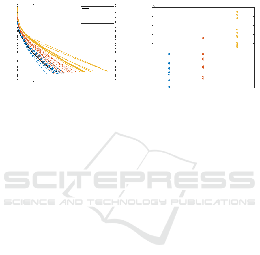
The differences of iteration numbers necessary to
converge to stationary points are shown in Figure 1.
The horizontal axis is iteration number and the ver-
tical axis is objective value. From Figure 1, we can
see that if we run our algorithm from initial points
generated by perturb + SKKR and low rank rand, it
converged faster than from an initial point provided
by SKKR. On the other hand, it took much more time
to converge if it started from initial points generated
by rand.
The objective values at the resulting stationary
points are shown in Figure 2. The vertical axis is
objective value. The black horizontal line around
perturb + SKKR low rank rand rand
0.8
1
1.2
1.4
1.6
1.8
2
2.2
2.4
2.6
objective value
10
-5
Figure 2: Comparison of objective values.
2 × 10
−5
depicts the objective value of the stationary
point provided by our algorithm starting from an ini-
tial point generated by SKKR. From Figure 2, we can
see that all solutions provided by our algorithm start-
ing from initial points generated by perturb + SKKR
and low rank rand are better than that by SKKR. Some
solutions resulting from rand is also smaller than that
from SKKR.
6 CONCLUSION
In this paper, we proposed a low-rank matrix approx-
imation model for completing a matrix with missing
values. Our proposed model utilizes not only a rank
constraint but also a box constraint. Owing to the
box constraint, this model shows promise for use in
recommendation systems. In addition, we proposed
an alternating minimization algorithm for solving our
proposed model, and proved that a sequence gener-
ated by our proposed algorithm converges to a sta-
tionary point under a mild assumption. Our numerical
results are preliminary, however, we showed that our
proposed algorithm converges quickly and provides
better solution than the existing method proposed by
Sarwar et al. (2000) in a specific case. The perfor-
mance of our algorithm depends on an initial guess.
Hence, we should try multiple initial guesses and take
the best one. In our experiments, we fixed parame-
ters r and λ. However, we should employ cross vali-
dation to decide appropriate values for such parame-
ters. We left extensive numerical experiments as our
future work.
Box Constrained Low-rank Matrix Approximation with Missing Values
83

ACKNOWLEDGEMENTS
We thank to Prof. Tomomi Matsui and anonymous
referees for providing helpful and useful comments,
respectively.
REFERENCES
Cand
´
es, E. J. and Recht, B. (2009). Exact matrix comple-
tion via convex optimization. Foundations of Compu-
tational Mathematics, 9(6):717–772.
Gillis, N. and Glineur, F. (2011). Low-rank matrix ap-
proximation with weights or missing data is NP-hard.
SIAM Journal on Matrix Analysis and Applications,
32(4):1149–1165.
Golub, G. H. and van Loan, C. F. (2013). Matrix Compu-
tations. The Johns Hopkins University Press, fourth
edition.
Ilin, A. and Raiko, T. (2010). Practical approaches to
principal component analysis in the presence of miss-
ing values. Journal of Machine Learning Research,
11(Jul):1957–2000.
Olsson, C. and Oskarsson, M. (2009). A convex approach
to low rank matrix approximation with missing data.
In Salberg, A.-B., Hardeberg, J. Y., and Jenssen, R.,
editors, Proceedings of the 16th Scandinavian Confer-
ence on Image Analysis (SCIA ’09), pages 301–309.
Sarwar, B., Karypis, G., Konstan, J., and Riedl, J. (2000).
Application of dimensionality reduction in recom-
mender system—a case study. In Kohavi, R., Masand,
B., Spiliopoulou, M., and Srivastava, J., editors, Pro-
ceedings of the ACM WEBKDD 2000 Workshop.
Su, X. and Khoshgoftaar, T. M. (2009). A survey of col-
laborative filtering techniques. Advances in Artificial
Intelligence, 2009(421425):1–19.
Tipping, M. E. and Bishop, C. M. (1999). Probabilistic prin-
cipal component analysis. Journal of the Royal Statis-
tical Society. Series B, 61(3):611–622.
Trefethen, L. N. and Bau, D. (1997). Numerical Linear
Algebra. SIAM.
Tseng, P. (2001). Convergence of a block coordinate
descent method for nondifferentiable minimization.
Journal of Optimization Theory and Applications,
109(3):475–494.
ICORES 2018 - 7th International Conference on Operations Research and Enterprise Systems
84
