Block based Spectral Processing of Dense 3D Meshes using Orthogonal
Iterations
Aris S. Lalos, Gerasimos Arvanitis, Anastasios Dimas and Konstantinos Moustakas
Department of Electrical and Computer Engineering, University of Patras, Patras, Greece
Keywords:
Graph Signal Processing, Mesh Compression, Mesh Denoising.
Abstract:
Spectral methods are widely used in geometry processing of 3D models. They rely on the projection of the
mesh geometry on the basis defined by the eigenvectors of the graph Laplacian operator, becoming compu-
tationally prohibitive as the density of the models increases. In this paper, we propose a novel approach for
supporting fast and efficient spectral processing of dense 3D meshes, ideally suited for real time compression
and denoising scenarios. To achieve that, we apply the problem of tracking graph Laplacian eigenspaces via
orthogonal iterations, exploiting potential spectral coherences between adjacent parts. To avoid perceptual
distortions when a fixed number of eigenvectors is used for all the individual parts, we propose a flexible
solution that automatically identifies the optimal subspace size for satisfying a given reconstruction quality
constraint. Extensive simulations carried out with different 3D meshes in compression and denoising setups,
showed that the proposed schemes are very fast alternatives of SVD based spectral processing while achieving
at the same time similar or even better reconstruction quality. More importantly, the proposed approach can
be employed by several other state of the art denoising methods as a preprocessing step, optimizing both their
reconstruction quality and their computational complexity.
1 INTRODUCTION
In recent years, there has been increasing interest
from researchers, system designers, and application
developers on acquiring, processing, transmitting and
storing 3D models, facilitating several real time ap-
plications, e.g., mobile cloud gaming (Cai et al.,
2013) and 3D Tele-immersion (Alexiadis et al., 2013;
Mekuria et al., 2014). These models usually come
as very large and noisy meshes that stand in need of
solutions for a diversity of problems including mesh
compression, smoothing, symmetry detection, wa-
termarking, surface reconstruction, and re-meshing
(Zhang et al., 2010). Spectral methods have been
developed with the intention of solving such prob-
lems by manipulating the eigenvalues, eigenvectors,
eigenspace projections, or a combination of these, de-
rived from the graph Laplacian operator. The pro-
cessing and memory requirements of these methods
are strongly dependent on the number of vertices of
the 3D model, and therefore become prohibitive as
the vertex density increases, especially in cases where
the models are too large and need to be canned in
parts, generating a sequence of 3D surfaces that ar-
rive sequentially in time. To address this issue, the
raw geometry data could be divided and processed
in blocks that represent the different parts of a mesh
(submeshes), as suggested in (Lalos et al., 2017; La-
los et al., 2015).
The application of direct singular value decom-
position (SVD) on the graph Laplacian of each sub-
mesh, requires O

n
3
d

operations, where n
d
is the
number of vertices in a submesh. This excessively
high computational complexity needed by SVD mo-
tivated us to seek for an efficient subspace tracking
implementation that processes the raw geometry data
in blocks and readjust only a small number of spec-
tral coefficients of a submesh based on the corre-
sponding spectral values of a previous submesh. The
proposed approach, is based on a numerical analysis
method known as orthogonal iterations (OI) (Zhang,
2009), which is capable of estimating iteratively the
subspaces of interest. The speed-up is attributed to
the fact that the proposed approach requires O

n
d
c
2

floating point operations where c is the number of
spectral components utilized and c << n
d
. Addition-
ally, we developed a dynamic OI approach that esti-
mates automatically the ideal c for a predefined recon-
struction quality. Extensive simulations carried out
with different 3D meshes in a compression and de-
noising setup, proved that the proposed framework is
a very fast alternative of the SVD based graph Lapla-
122
Lalos, A., Arvanitis, G., Dimas, A. and Moustakas, K.
Block based Spectral Processing of Dense 3D Meshes using Orthogonal Iterations.
DOI: 10.5220/0006611401220132
In Proceedings of the 13th International Joint Conference on Computer Vision, Imaging and Computer Graphics Theory and Applications (VISIGRAPP 2018) - Volume 1: GRAPP, pages
122-132
ISBN: 978-989-758-287-5
Copyright © 2018 by SCITEPRESS – Science and Technology Publications, Lda. All rights reserved

cian processing methods, without introducing notice-
able reconstruction errors.
The rest of the article is organized as follows. Sec.
II provides a review of prior art on spectral methods
and their applications in a diversity of problems. Ba-
sic definitions related to graph spectral processing of
3D meshes are provided in Sec. III. Sec. IV presents
the proposed fast spectral processing approach that is
based on OI. Section V provides a flexible solution
that automatically identifies the optimal subspace size
c that satisfies a specific reconstruction quality crite-
rion. Section VI presents a compression and a denois-
ing case study, where the proposed method can be ef-
fectively adopted. In Section VII, the performance of
the proposed system is evaluated, by taking into ac-
count different CAD and scanned 3D models. The
article is finally wrapped up with a few open research
directions in Sec. VIII.
2 RELATED WORKS
Spectral methods have been used in many different
computer science fields ranging from signal process-
ing, graph theory, computer vision and machine learn-
ing. Spectral mesh processing have been inspired by
all the relevant developments in the aforementioned
fields. Several surveys that cover basic definitions
and applications of the graph spectral methods have
been introduced by Gotsman (Gotsman, 2003), Levy
(L
´
evy, 2006), Sorkine (Sorkine, 2005) and more re-
cently by Zhang et al. (Zhang et al., 2010). All
these surveys classify the spectral methods according
to several criteria related to the employed operators,
the application domains and the dimensionality of the
spectral embeddings used.
Graph spectral processing of 3D meshes rely on
the singular/eigen-vectors and/ or eigenspace projec-
tions derived from appropriately defined mesh opera-
tors, while it has been applied in several tasks, such
as, implicit mesh fairing (Kim and Rossignac, 2005),
geometry compression (Sorkine, 2005; Karni and
Gotsman, 2000) and mesh watermarking (Ohbuchi
et al., 2001). Taubin (Taubin, 1995) first treated the
mesh vertex coordinates as a 3D signal and intro-
duced the use of graph Laplacian operators for dis-
crete geometry processing. This analysis was moti-
vated by the similarities between the spectral analy-
sis with respect to mesh Laplacian and the classical
Fourier analysis. A summary of the mesh filtering
approaches that can be efficiently carried out in the
spatial domain using convolution approaches is given
by Taubin in (Taubin, 2000). Despite their applica-
bility in a wide range of applications such as, mesh
denoising, geometry compression and watermarking,
they require explicit eigenvector computations mak-
ing them prohibitive for real time scenarios such as
streaming and content creation applications, where
large 3D models are generated in parts, providing a
sequence of 3D surfaces that need to be processed fast
and sequentially in time.
Computing the truncated singular value decom-
position, can be extremely memory-demanding and
time-consuming. To overcome this limitations, sub-
space tracking algorithms have been proposed as
fast alternatives relying on the execution of iterative
schemes for evaluating the desired eigenvectors per
incoming block of floating point data corresponding
in our case, to different surface patches (Comon and
Golub, 1990). The most widely adopted subspace
tracking method is Orthogonal iterations (OI), due to
the fact that results in very fast solutions when the ini-
tial input subspace is close to the subspace of interest,
as well as the size of the subspace remains at small
levels (Saad, 2016). The fact that both matrix multi-
plications and QR factorizations have been highly op-
timized for maximum efficiency on modern serial and
parallel architectures, makes the OI approach more at-
tractive for real time applications. To the best of our
knowledge, subspace tracking algorithms have never
been applied for graph spectral mesh processing, de-
spite their wide success on a large range of filtering
applications.
3 SPECTRAL PROCESSING OF
3D MESHES
In this work we focus on polygon models whose sur-
face is represented using triangles. Let us assume
that each triangle mesh M with n vertices can be
represented by two different sets M = (V,F) corre-
sponding to the vertices (V ) that represent the ge-
ometry information and the indexed faces (F) of the
mesh. Each vertex can be represented as a point
v
i
= (x
i
,y
i
,z
i
) ∀ i = 1,n and each centroid of a face
as m
i
= (v
i1
+ v
i2
+ v
i3
)/3 ∀ i = 1,l. A set of edges
(E) can be directly derived from V and F, which cor-
respond to the connectivity information.
Spectral processing approaches, e.g., (Sorkine,
2005; Karni and Gotsman, 2000) are based on the fact
that smooth geometries should yield spectra, domi-
nated by low frequency components and suggest pro-
jecting the Cartesian coordinates x,y, z ∈ ℜ
n×1
in the
basis spanned by the eigenvectors u
i
, i = 1,..., c << n
of the Laplacian operator L that is calculated as fol-
lows:
L = D − C, (1)
Block based Spectral Processing of Dense 3D Meshes using Orthogonal Iterations
123

where C ∈ ℜ
n×n
is the weighted connectivity matrix
of the mesh with elements:
C
(i, j)
=
(
1
kv
i
−v
j
k
2
2
(i, j) ∈ (E)
0 otherwise,
, (2)
matrix D is the diagonal matrix with D
(i,i)
=
|
N(i)
|
,
and N(i) =
{
j
|
(i, j) ∈ (E)
}
is a set of the immediate
neighbors for node i. The weighted adjacency ma-
trix is ideal for emphasizing the coherence between
Laplacian matrices of different submeshes by provid-
ing geometric information; on the contrary, the binary
provides only connectivity information. Eigenvalue
decomposition of L is written as:
L = UΛU
T
(3)
where Λ is a diagonal matrix consisting of the eigen-
values of L and U = [u
1
,.. .,u
n
] is the matrix with the
eigenvectors u
i
∈ ℜ
n×1
which is needed to generate
the spectral coefficients that are essential in provid-
ing sparse representations of the raw geometry data
(Sorkine, 2005).
Similar to classical Fourier transform, the eigen-
vectors and eigenvalues of the Laplacian matrix L
provide a spectral interpretation of the 3D signal.
The eigenvalues
{
λ
1
,λ
2
,.. .,λ
n
}
can be considered as
graph frequencies, and the eigenvectors demonstrate
increasing oscillatory behavior as the magnitude of
λ
i
increases (BrianDavies et al., 2001). The Graph
Fourier Transform (GFT) of the vertex coordinates is
defined as its projection onto the eigenvectors of the
graph, i.e.,
¯
v = U
T
v and the inverse GFT is given by
v = U
¯
v.
4 BLOCK BASED SPECTRAL
PROCESSING USING OI
As mentioned earlier, calculating the graph Laplacian
eigenvalues of the mesh geometry can become restric-
tive as the density of the models increases. To over-
come this limitation, several approaches suggest pro-
cessing large meshes into parts (Cayre et al., 2003;
Lalos et al., 2015). Thus, we assume the original 3D
mesh is partitioned into k non-overlapping parts using
the MeTiS algorithm described in (Karypis and Ku-
mar, 1998). Processing of a single mesh in parts usu-
ally results in a loss of reconstruction quality that is
attributed to the dislocation of the vertices that lie on
the edges of each sub mesh. These phenomena, also
known as edge effects, can be mitigated by process-
ing overlapped submeshes (Cayre et al., 2003; Lalos
et al., 2015). Therefore each submesh is extended
with the neighbors of the boundary nodes of adjacent
submeshes consisting in total of n
d
nodes. This op-
eration reduces the error introduced when increasing
the number of sub meshes.
The evaluation of the eigenvectors of the respec-
tive matrix L[i] ∀i = 1,..., k requires O(kn
3
d
) floating
point operations. To minimize this complexity, we
suggest exploiting the coherence between the spec-
tral components of the different submeshes using OI
(Golub and Van Loan, 2012). This assumption is
strongly based on the observation that submeshes of
the same mesh maintain similar geometric character-
istics and connectivity information.
The Orthogonal Iteration is an iterative procedure,
that can be used to compute the singular vectors cor-
responding to the dominant singular values of a sym-
metric, nonnegative definite matrix. Alternatively, to
the OI one could use Lanczos approach. However,
the initialization of OI to a starting subspace close
to the subspace of interest leads to a very fast solu-
tion. This property is efficiently exploited when pro-
cessing sequential submeshes, leading to a lower to-
tal complexity as compared to the complexity of the
Lanczos approach. Building on this line of thought
we suggest evaluating the c eigenvectors correspond-
ing to the c lowest eigenvalue of L[i] each submesh i,
U
c
[i] = [u
1
,.. .,u
c
] ∈ ℜ
n
d
×c
according to Algorithm
1, where R
i
= (L[i] + δI)
−1
and δ is a small positive
Algorithm 1: OI update process for each submesh
i (OI).
1 U(0) ← U
c
[i −1];
2 for t ← 1 to t
max
do
3 U(t) ← Onorm(R
z
i
U(t − 1));
4 end
5 U
c
[i] ← U(t);
scalar value that ensures positive definiteness of R
i
.
Matrix I is the identity matrix of size n
d
× n
d
. At this
point it should be noted that the projected coefficients
R
z
i
U(t − 1) are estimated very efficiently using sparse
linear system solvers (Sorkine, 2005). Depending
on the choice of power value z, we obtain alterna-
tive iterative algorithms with different convergence
properties. The convergence rate of OI depends on
|λ
c+1
/ λ
c
|
z
where λ
c+1
is the (c + 1)-st largest eigen-
value of R
i
(Zhang, 2009). To preserve orthonormal-
ity, it is important that the initial subspace
e
U
c
[0] is or-
thonormal. For that reason,
e
U
c
[0] is estimated by ap-
plying SVD directly on the first selected sub mesh
1
,
while the following subspaces
e
U
c
[i], i = 2, .. .,k are
adjusted using Algorithm 1. The initial submesh is
1
Please note that the selection of the initial sub mesh
does not affect the transient behavior of the algorithm
GRAPP 2018 - International Conference on Computer Graphics Theory and Applications
124

selected in a random order and the subsequent ones
are processed in a topologically sorted order.
The orthonormalization of the estimated sub-
space can be performed using a number of differ-
ent choices(Hua, 2004) that affect both complexity
and performance.The most widely adopted are the
Householder Reflections (HR), Gram-Schmidt (GS)
and Modified GramSchmidt (MGS) methods. Al-
though, the aforementioned variants exhibit differ-
ent properties related to the numerical stability and
computational complexity, the Onorm(·) step is per-
formed using HR.
5 DYNAMIC OI FOR STABLE
RECONSTRUCTION
In application scenarios where the original mesh is
known, we propose a flexible solution that automat-
ically identifies the optimal subspace size c that sat-
isfies a specific reconstruction quality criterion. This
novel extension can be used for improving the recon-
struction quality in special cases where the coherence
between submeshes is not strong enough e.g. differ-
ent density, difference in geometry. The identifica-
tion is performed sequentially, based on user defined
thresholds, that determine the lower and higher ”ac-
ceptable” quality of the reconstructed submeshes at
the decoder side. In practical scenarios it is reason-
able to assume that the feature vectors E[i] = U
T
c
[i]v[i]
of each block v[i] ”live” in subspaces U
c
[i] of differ-
ent sizes. The subspace size c
i
of the incoming data
block v[i], should be carefully selected so that the rel-
evant submesh vertices are identified with the min-
imum loss of information. To quantify this loss at
each iteration t, we suggest using the l
2
-norm of the
following mean residual vector:
e(t) =
∑
j∈
{
x,y,z
}

v
j
[i] − U
c
[i]U
T
c
[i]v
j
[i]

(4)
where each v
j
[i], ∀
{
x,y,z
}
correspond to the n
d
× 1
vector with the x,y and z coordinates of the submesh
i vertices. When the l
2
norm value of this metric is
below a given threshold ke(t)k
2
< ε
h
the loss of in-
formation during the spectral processing steps is not
easily perceived. To reduce the residual error e(t),
we suggest adding one normalized column in the es-
timated subspace U
c
(t) = [U
c
(t − 1) e(t − 1)/ke(t −
1)k
2
] and then perform orthonormalization, e.g.,
U
c
(t) = Onorm

R
z
[i][U
c
(t −1)
e(t −1)
ke(t −1)k
2
]

(5)
Similarly, when the value of the reconstruction
quality metric is less than a user determined lower
bound ε
l
the subspace size is decreased by 1 by sim-
ply selecting the first c
i
− 1 columns of U
c
(t). This
procedure is repeated until the value of the metric
lies within the range (ε
l
,ε
h
), allowing the user to
easily trade the reconstruction quality with the com-
putational complexity. To summarize, Algorithm 2
presents the steps of the dynamic OI approach.
Algorithm 2: Dynamic OI for each submesh i
(DOI).
1 U(0) = U
i−1
;
2 c
i
← (i > 0) ? c
i−1
: c;
3 for t = 1, 2, ... do
4 U(t) = [u
1
...u
c
t
] = Onorm(R
z
i
U(t − 1));
5 e(t) =
∑
j∈
{
x,y,z
}

v
i j
− U(t)U(t)
T
v
i j

;
6 if ke(t)k
2
< ε
l
then
7 U(t) = [U(t −1)
e(t)
ke(t)k
2
]; c
i
← c
i
+ 1;
8 else if ke(t)k
2
> ε
h
then
9 U(t) = [u
1
...u
c
t
]; c
i
← c
i
− 1;
10 else
11 break;
12 end
13 end
14 U
i
= U(t);
6 APPLICATIONS
The primary purpose of this work is the creation of
a framework for fast and effective spectral processing
of large 3D meshes. In this section we present two
case studies a) compression, b) denoising where the
proposed schema can be applied.
6.1 Block based Spectral Compression
of 3D Meshes
The spectral compression and reconstruction of static
meshes utilize the subspace
e
U
c
[i] for encoding and
decoding the raw geometry data. During the en-
coding step, the dictionary
e
U
c
[i] is evaluated, either
by direct SVD or by executing a number of OI on
R
z
[i], and is used for providing a compact represen-
tation of the Euclidean coordinates of each submesh,
e.g. for coordinates v
x
[i] ∈ ℜ
n
d
×1
, E [i] = U
T
c
[i]v[i],
where E[i] ∈ ℜ
c×1
and c << n
d
i
. At the decoder side
the original 3D vertices of each submesh are recon-
structed from the feature vector E[i] and the dictio-
nary U
c
[i] according to :
˜
v[i] = U
c
[i]E[i]. Note that
the subspace size c remains fixed in the OI case, sat-
isfying fast streaming scenarios, while DOI approach
aims at providing high and stable reconstruction ac-
curacy. It is important to mention that the only in-
formation transmitted from the sender is the connec-
Block based Spectral Processing of Dense 3D Meshes using Orthogonal Iterations
125

bpv
2 3 4 5 6 7 8 9 10 11 12
NMSVE (dB)
-54
-53
-52
-51
-50
-49
-48
-47
-46
-45
10.72 sec. !
1.14 sec. !
0.81 sec. !
0.5 sec. !
5.94 sec. !
0.47 sec. !
Dense Mesh Compression (Bunny)
Identity
OI (t=1, z=1)
OI (t=2, z=1)
OI (t=1, z=2)
SVD
DOI (9e-5,4e-5)
(a)
Number of eigenvectors
50 100 150 200 250 300
NMSVE (dB)
-49
-48
-47
-46
-45
-44
-43
-42
-41
-40
13.68 sec. !
0.66 sec. !
0.57 sec. !
0.32 sec. !
0.24 sec. !
Original
Mesh
Partitioned
Original
with
Noise
Dense Mesh Denoising (Armadillo)
Identity
OI (t=1, z=1)
OI (t=2, z=1)
OI (t=1, z=2)
SVD
(b)
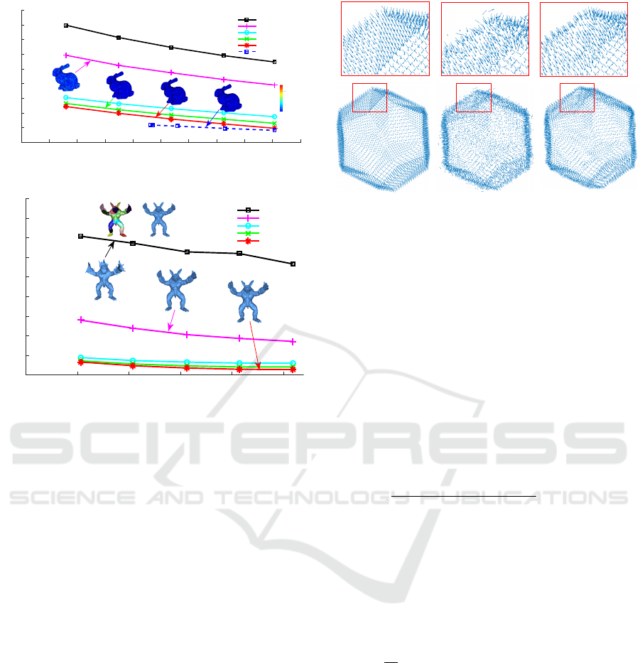
Figure 1: (a) Compression Study: NMSVE vs bpv for
the Bunny model (34,817 vertices) was partitioned into 70
blocks with about 512 vertices per block. (b) Coarse-to-
fine Denoising study using the Armadillo model (20,002
vertices) was partitioned into 20 submeshes each compris-
ing of around 990 vertices with zero-mean Gaussian noise
N (0,0.2).
tivity of the mesh and the c respective spectral co-
efficients of each block. At the receiver’s side, the
dictionary
e
U
c
[i] is evaluated utilizing the connectivity
information. For the decoding process, the received
spectral coefficients and the dictionary are used to re-
trieve the original Euclidean coordinates
ˆ
x
i
,
ˆ
y
i
,
ˆ
z
i
, e.g.
ˆ
x
i
=
e
U
c
[i]s
x
i
. Spectral compression enables aggres-
sive compression ratios, without introducing a signif-
icant loss on the visual quality (Karni and Gotsman,
2000).
6.2 Block based Spectral Denoising of
3D Meshes
Bilateral techniques have been used as mesh denois-
ing method in many studies (Fleishman et al., 2003),
(Zheng et al., 2011), (Zhang et al., 2015) by iter-
atively adjusting the face normals and vertices. In
this section, we suggest executing a coarse-to-fine
spectral denoising method that initially filters out the
high spectral frequencies using the aforementioned
(a)
(b)
(c)
Figure 2: (a) Normals vector of original mesh, (b) Normals
vector of noisy mesh, (c) Smoothed normals vector.
approach and then performs a fine denoising step us-
ing a two stage bilateral technique. The use of the
coarse step significantly accelerates the convergence
of the fine since it filters out the noise that appears in
the higher frequencies, providing a set of normal vec-
tors that are closer to the normal vectors of the origi-
nal model, as it is clearly shown in the dodecahedron
model Fig. 2.
We finally show that the fine technique can be also
considered as Graph Spectral Processing approach. If
we denote with
ˆ
v[i] = U
c
U
T
c
v[i] the vertices of the
coarse denoised i submesh, then each face can be rep-
resented by its centroid point m
i
, and its outward unit
normal:
ˆ
n
m
i
=
(
ˆ
v
i
2
−
ˆ
v
i
1
) × (
ˆ
v
i
3
−
ˆ
v
i
1
)


(
ˆ
v
i
2
−
ˆ
v
i
1
) × (
ˆ
v
i
3
−
ˆ
v
i
1
)


∀ i = 1,n
f
. (6)
where
ˆ
v
i
1
,
ˆ
v
i
2
,
ˆ
v
i
3
are the vertices that are related with
face f
i
and
ˆ
n
m
= [
ˆ
n
T
m
1
ˆ
n
T
m
2
···
ˆ
n
T
n f
] ∈ ℜ
3n
f
×1
.
The bilateral technique estimates the new face
normals n
i
using a normal guidance unit vector g
i
,
which it is calculated as a weighted average of nor-
mals in a neighborhood of i is computed by:
ˆ
n
m
i
=
1
W
i
∑
f
j
∈N
f
i
A
j
K
s
(m
i
,m
j
)K
r

n
m
i
,n
m
j

n
m
j
(7)
where N
f
i
is the set of faces in a neighborhood of
f
i
, A
j
is the area of face f
j
, W
i
is a weight that en-
sures that
ˆ
n
m
i
is a unit vector and K
s
, K
r
are the spatial
and range Gaussian kernels. More specifically, K
s
is
monotonically decreasing with respect to the distance
of the centroids m
i
and m
j
which lie on the mesh sur-
face, while K
r
is monotonically decreasing with the
proximity of the guidance normals that lie on the unit
sphere:
GRAPP 2018 - International Conference on Computer Graphics Theory and Applications
126

K
s
(m
i
,m
j
) = exp −


m
i
− m
j


2
2σ
2
s
!
, (8)
K
r

n
m
i
,n
m
j

= exp −


n
m
i
− n
m
j


2
2σ
2
r
!
(9)
The Bilateral filter output is then used to update
the vertex positions in order to match the new normal
directions n
m
i
, according to the iterative scheme pro-
posed in (Zhang et al., 2015). More specifically, the
vertex positions
ˆ
v
i
1
,
ˆ
v
i
2
,
ˆ
v
i
3
of a face f
i
are updated in
an iterative manner, according to:
ˆ
v
(t+1)
i
j
=
ˆ
v
(t)
i
j
+
1



F
i
j



∑
z∈F
i
j
ˆ
n
m
z
h
ˆ
n
T
m
z

m
(t)
i
−
ˆ
v
(t)
i
j
i
(10)
m
(t)
i
=

ˆ
v
(t)
i
1
+
ˆ
v
(t)
i
2
+
ˆ
v
(t)
i
3

/3 (11)
where (t) denotes the iteration number, F
i
j
is the
index set of incident faces for
ˆ
v
i
j
. This iterative pro-
cess can be considered as a gradient descent process
that is executed for minimizing the following energy
term across all faces
∑
z∈F
i
j



ˆ
n
T
m
z

m
(t)
i
−
ˆ
v
(t)
i
j




2
, j = 1, 2,3. (12)
This term penalizes displacement perpendicular to
the tangent plane defined by the vertex position
ˆ
v
(t)
i
j
and the local surface normal
ˆ
n
m
z
Bilateral filter as a graph based transform:
Consider an undirected graph G = (V ,E) where
the nodes V =
{
1,2,. .., n
}
are the normals n
m
i
, as-
sociated with the centroids m
i
and the edges E =

(i, j,c
i j
)

capture the similarity between two nor-
mals as given by the bilateral weights in eq. (8),
(9). The input normals can be considered as a sig-
nal defined on this graph n
i
: V → ℜ
3×1
where the
signal value at each node correspond to the normal
vector. Let C be the adjacency matrix with the bilat-
eral weights and D = diag
n
W
1
,.. .,W
n
f
o
the diago-
nal degree matrix, then eq. (7) can be written as:
ˆ
n = D
−1
Cn
= D
−1/2
D
−1/2
CD
−1/2
D
1/2
n
D
1/2
ˆ
n = (I − L)D
1/2
n
D
1/2
ˆ
n = U
|{z}
IGFT
(I − Λ)
| {z }
Spectral
response
U
T
|{z}
GFT
D
1/2
n. (13)
Thus, it is clearly shown that the Bilateral fil-
ter can be considered as a frequency selective graph
transform with a spectral response that corresponds
to a linear decaying function, meaning that it tries to
preserve the low frequency components and attenuate
the high frequency ones.
7 PERFORMANCE EVALUATION
In the following section, we evaluate the presented
framework in two different case studies: i) block
based mesh compression and ii) block based mesh de-
noising, that effectively take advantage of the spectral
coherence between different blocks utilizing OI. Each
case study is examined using a static large (≥ 2 · 10
4
vertices) and very large (≥ 1 · 10
6
vertices) mesh
partitioned using MeTis. All simulations were per-
formed on an Intel Core i7-4790 (3.6 GHz) proces-
sor with 8GB RAM. The compression efficiency of
the geometry is measured in bits-per-vertex (bpv =
3·q
c
·c ·k/n
d
) where q
c
are the bits used for uniformly
quantizing the feature vectors (q
c
= 12 bits) and c
the total components kept from each submesh. This
metric encapsulates the feature vectors for each pro-
cessed block, ignoring the mesh connectivity which
can be effectively compressed through any state-of-
the-art connectivity encoder (Rossignac, 1999). To
evaluate the reconstruction quality of our proposed
method, it is necessary to capture the distortion be-
tween the original and the approximated frame. For
this task, we chose the normalized mean square vi-
sual error (NMSVE) (Karni and Gotsman, 2000) cal-
culated as:
1
2n

k
v −
˜
v
k
l
2
+
k
GL (v) − GL (
˜
v)
k
l
2

(14)
where GL(v
i
) = v
i
− (
∑
j∈N(i)
d
−1
i j
v
j
)/(
∑
j∈N(i)
d
−1
i j
),
v,
˜
v ∈ R
3n×1
represent vectors that contain the orig-
inal and reconstructed vertices respectively, and d
i j
denotes the Euclidean distance between i and j.
7.1 Compression Results
The NMSVE vs bpv results are shown in Fig. 1 (a)
for the Bunny model. Note that the execution times
shown next to each line encapsulate the respective
time needed to construct R
z
,z ≥ 1, and to run the re-
spective number of OI. By inspecting the figure, it can
be easily concluded that the quality of the OI method
performs almost the same as with SVD, especially
when the number of iterations increases. At this point
it should be noted that the benefits of our method are
directly related to the size of each block. The theo-
retical complexities of the proposed schemes are in
tandem with the measured times. More specifically,
Block based Spectral Processing of Dense 3D Meshes using Orthogonal Iterations
127

the OI approach for the Bunny mesh can be executed
up to 20 times faster than the direct SVD approach.
Although running more OI iterations yields a better
NMSVE, converging towards the (optimal) SVD re-
sult, it comes at the cost of a linear increase in the
decoding time. On the other hand, one iteration of
R
2
achieves lower visual error as executing two OI,
in considerably less time. Moreover, DOI provides
a stable reconstruction accuracy (see Fig. 3 showing
the per submesh error) that can easily be adjusted by
the defined thresholds. By inspecting also Fig. 3, it is
obvious that there is a coherence between submeshes
since there are very few abrupt changes in the ’ideal’
value of subspace size that is required to satisfy a pre-
defined reconstruction quality.
Number of Submesh
0 10 20 30 40 50 60 70
Squared Error
-50
-40
-30
-20
-10
0
Bunny (70 Submeshes of 512 vertices)
SVD
OI
OI (t=1, z=2)
DOI
Submesh 11 Submesh 27
Submesh 46
Number of Submesh
0 10 20 30 40 50 60 70
Ideal Number of c
420
440
460
480
500
c
0
= 460, (0
h
= 2e-4, 0
l
= 1.8e-4)
c
0
= 435, (0
h
= 3e-4, 0
l
= 2.8e-4)
c
0
= 409, (0
h
= 4e-4, 0
l
= 3.8e-4)
11
27
46
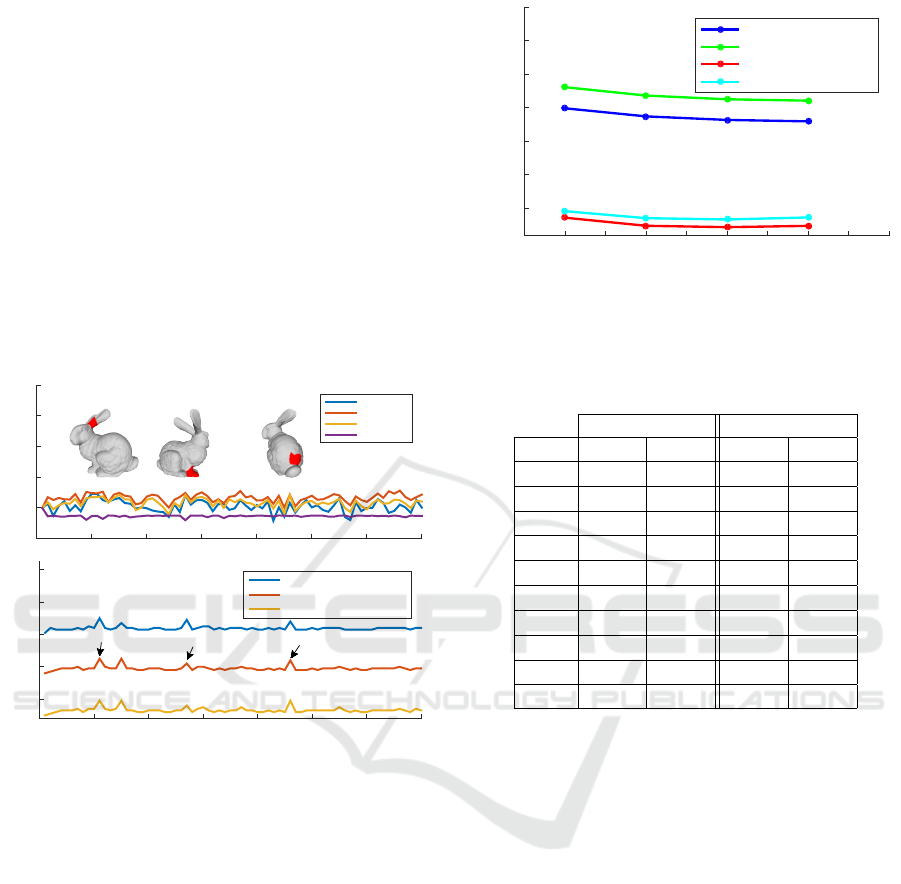
Figure 3: [Up] Squared Error per submesh for different ap-
proaches. [Bottom] Ideal value c of subspace size per sub-
mesh.
However, this comes with a slight increase on the exe-
cution time (more OI) as well as a significant increase
on the final compression rate (bpv) captured in Fig. 1
(a) as a right shifting of the plot. The shifting is more
obvious when the initial value of c is small (more
OI iterations are necessary for achieving the accuracy
threshold).
7.2 Denoising Results
Similar conclusions are also drawn in a coarse-to-fine
denoising setup where OI method are used as a pre-
processing, ”smoothing” step, before applying a con-
ventional spectral bilateral filtering Fig. 1 (b). Fig. 4
shows the effects of the coarse denoising step in the
execution time of the guided mesh approach (Zhang
et al., 2015). By inspecting the number of iterations
required for achieving a given reconstruction quality,
Number of Bilateral Iterations
5 10 15 20 25 30 35 40 45 50
NMSVE (dB)
-46.5
-46
-45.5
-45
-44.5
-44
-43.5
u
iter
= 30
u
iter
= 40
u
iter
= 30 with preprocessing
u
iter
= 40 with preprocessing
Figure 4: Coarse denoising step increases the reconstruc-
tion quality. In other words, less faces/vertices updates are
required in order to achieve the same quality.
Table 1: Execution time and face angle difference θ for dif-
ferent cases of R
z
and SVD.
Twelve Fandisk
t θ t θ
R
1
0.031 11.57 0.077 16.36
R
2
0.049 10.26 0.110 14.75
R
3
0.099 13.97 0.170 14.54
R
4
0.114 13.84 0.202 14.54
R
5
0.136 13.7 0.242 14.44
R
6
0.142 13.59 0.297 14.5
R
7
0.157 13.57 0.313 14.52
R
8
0.184 13.55 0.355 14.84
R
9
0.201 13.53 0.407 15.6
SVD 0.901 9.83 1.953 14.56
it can be easily noted that the coarse denoising step
accelerates the convergence rate of the fine denoising
approach, thus significantly improving the total exe-
cution time of the whole denoising process.
In Figs. 5 and 6, it can be easily observed that the
presented OI method can be employed by any other
state-of-the-art (SoA) denoising method as a prepro-
cessing step (Zheng et al., 2011; He and Schaefer,
2013; Zhang et al., 2015), optimizing both its recon-
struction quality and its computational complexity.
The use of the coarse step significantly accelerates the
convergence of the fine reducing the face/vertex up-
date iterations required for achieving a specific recon-
struction quality.The reconstruction benefits can be
easily identified by inspecting Fig. 5 which presents
denoising results of SoA methods (first row) and the
corresponding results after using the OI approach as a
preprocessing step (second row).
Moreover, we also examined different combina-
tions of z (power of R) and number of iterations in
the denoising setup. Figure 7 shows the results of
the coarse denoising step using OI for different val-
ues of z. Higher values, result in higher accuracies as
GRAPP 2018 - International Conference on Computer Graphics Theory and Applications
128

(Ι)
(II)
(III) (IV) (V)
Denoising
Denoising
Denoising
& GSP
Denoising
& GSP
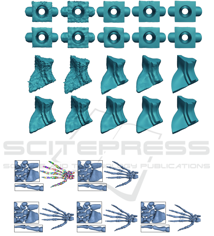
Figure 5: Coarse denoising improves the efficiency of the following SoA approaches: (i) bilateral (Fleishman et al., 2003),
(ii) non iterative (Jones et al., 2003), (iii) fast and effective (Sun et al., 2007), (iv) bilateral normal [24], (v) guided normal
filtering (Zhang et al., 2015) (zero-mean Gaussian noise N (0,0.7)).
Original mesh partitioned
Original with noise
SVD DOI (4.999e-12,2.999e-12)OI
700 submeshes
481 vertices
Original mesh partitioned
Original with noise
SVD DOI (4.999e-12,2.999e-12)OI
700 submeshes
481 vertices
Figure 6: Graph Spectral processing of Hand (327,323 vertices) using c = 47 eigenvectors, by applying the (a) OI method,
(b) traditional SVD method, (c) Dynamic OI method.
compared to the direct application of SVD. While it
should be noted that for z > 4 the results are identi-
cal identical with that achieved by applying the direct
SVD.
We evaluated the effects of executing several OI
either on R
z
or on R in CAD and scanned 3D mod-
els, using the NMSVE and the angle difference be-
tween the normal of the ground truth face and the
corresponding normal of the reconstructed face, av-
eraged over all faces (θ). The differences between
the SVD and OI, in terms of both reconstruction qual-
ity and execution time, are presented in Tables 1 and
2. It is clearly shown that the application of OI on
R
z
results in faster execution times than the applica-
Block based Spectral Processing of Dense 3D Meshes using Orthogonal Iterations
129

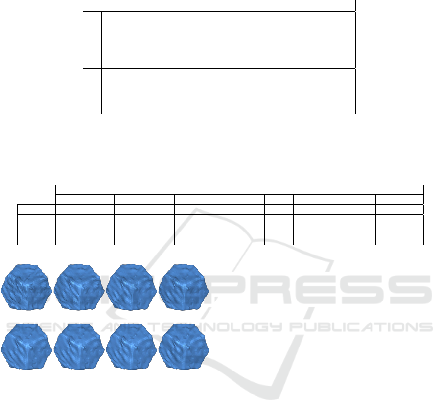
Table 2: NMSVE and Execution Times.
NMSVE (dB) Time (sec.)
ver/clust SVD OI SVD OI Speed-up
Armadillo
10% -47.5668 -47.4145 8.65 0.40 22x
15% -47.6641 -47.5263 8.80 0.53 16x
20% -47.7428 -47.6195 9.06 0.65 14x
25% -47.8301 -47.7097 9.16 0.80 12x
Hand
10% -59.0354 -58.8521 48.36 0.54 89x
15% -58.872 -58.7107 48.85 0.69 70x
20% -58.6218 -58.489 49.14 1.05 46x
25% -58.3314 -58.2215 49.53 1.31 37x
Table 3: Time performance for different models. k
iter
presents the number of iterations for bilateral filtering normal executed
in t
k
iter
, u
iter
is the number of iterations for vertex update executed in t
u
iter
and N is the number of points searched for finding
ideal patches (according to (Zhang et al., 2015)) executed in t
N
. t
cd
corresponds to execution time for coarse denoising,
features extraction and level noise estimation, t
cd
represents the execution time for fine denoising and t
tot
is the total time
expressed in seconds.
Guided normal filtering (GNF) (Zhang et al., 2015) GNF using Coarse denoising step
k
iter
t
k
iter
t
u
iter
N t
N
t
tot
t
cd
t
fn
t
u
iter
N t
N
t
tot
Block 40 200.31 21.88 17550 10.63 232.82 7.08 32.59 14.78 4457 2.68 57.13 -75%
Twelve 75 273.07 7.64 9216 8.11 289.55 2.25 18.67 11.54 2297 2.31 34.77 -88%
Sphere 30 106.91 17.60 20882 6.53 131.05 8.19 18.10 10.44 3635 1.22 37.95 -71%
Fandisk 50 257.13 10.61 12946 12.19 279.94 7.53 44.82 10.82 4464 4.34 67.51 -75%
(a) (b) (c) (d)
(e) (f) (g) (h)
Figure 7: Coarse denoising results for different cases of R
z
,
(a) z = 1 (b) z = 2 (c) z = 3 (d) z = 4 (e) z = 5 (f) z = 6 (g)
z = 7 (h) SVD.
tion on R. This result is attributed to the facts that: i)
the execution of OI on R requires z times more iter-
ations to converge than the execution on R
z
ii) while
the evaluation of a matrix-matrix product (e.g., R×R,
e.t.c.) is much less computationally demanding than
the orthonormalization step. These effects become
more apparent in dense models (see. Table 2). Fi-
nally, in Table 3 we present the execution times of
the proposed denoising approach as compared to the
Guided Mesh algorithm (Zhang et al., 2015), which
provided the best results among the SoA competitors.
Note that while both approaches, are based on a se-
quential update of the face normals and vertices, the
GNF with coarse denoising, results to lower execu-
tion times (12x-88x). This reduction is attributed to
the application of the coarse denoising step that fil-
ters out the high frequency components, accelerating
the convergence speed of the necessary corrections/
adjustments of the vertex positions.
8 DISCUSSION AND
CONCLUSION
In this paper, we introduced a fast and efficient way
of performing spectral processing of 3D meshes ide-
ally suited for real time applications. The proposed
approach apply the problem of tracking graph Lapla-
cian eigenspaces via orthogonal iterations, exploiting
potential spectral coherences between adjacent parts.
The thorough experimental study on a vast collection
of 3D meshes that represent a wide range of CAD and
scanned Models showed that the subspace tracking
approaches allow the robust estimation of dictionar-
ies at significantly lower execution times compared
to the direct SVD implementations. Despite the su-
periority of OI based approaches when compared to
the direct SVD, the optimal subspace size should be
carefully selected in order to simultaneously achieve
the highest reconstruction quality and fastest com-
pression times. One interesting future direction, is
to propose an automatic modeled based approach for
identifying the subspace size where the features lie
together with the level of noise. In addition, the ap-
proximation artifacts that occur in a single block may
GRAPP 2018 - International Conference on Computer Graphics Theory and Applications
130

Application of [30] in noisy
CAD model
Application of [30] in a GSP
processed CAD model
Application of [30] in a GSP
processed scanned model
Application of [30] in noisy
scanned model
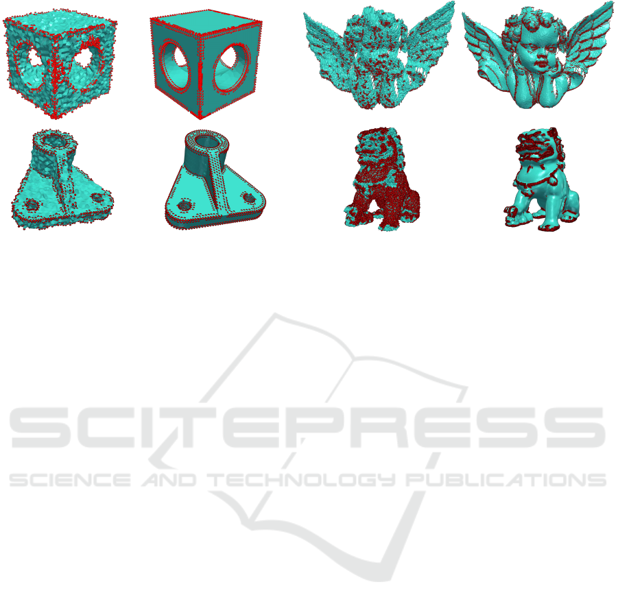
Figure 8: Identification of sharp and small scale geometric features in noisy objects with and without DAOI step.
slightly increased and propagated when moving to the
subsequent ones. To address the latter issue, we sug-
gest to either re-initialize the subspace of interest us-
ing the SVD or execute an DAOI update. At this point
we would like also to highlight another strong point
of the proposed GSP scheme. The proposed GSP ap-
proach increases significantly the accuracy of state of
the art schemes, focusing on identifying sharp and
small scale geometric features. In Fig. 8, we present
the identified features in the case that we use as input
a noisy model or the same noisy model after apply-
ing the GSP approach. It is clearly shown that the
GSP approach increases significantly the robustness
of the feature identification approach, allowing the ac-
curate detection of high frequency featurea that could
be further used by several feature aware compression,
completion and denoising approaches. Without any
doubt, the presented signal processing approaches are
expected to provide a novel insight at key areas, e.g.,
compression and feature preserving denoising where
high potential for novel improvements is feasible in
the near future.
REFERENCES
Alexiadis, D. S., Zarpalas, D., and Daras, P. (2013). Real-
time, full 3-D reconstruction of moving foreground
objects from multiple consumer depth cameras. IEEE
Transactions on Multimedia, 15(2):339–358.
BrianDavies, E., Gladwell, G. L., Leydold, J., and Stadler,
P. F. (2001). Discrete nodal domain theorems. Linear
Algebra and its Applications, 336(1-3):51–60.
Cai, W., Leung, V. C. M., and Chen, M. (2013). Next Gen-
eration Mobile Cloud Gaming. 2013 IEEE Seventh
International Symposium on Service-Oriented System
Engineering, pages 551–560.
Cayre, F., Rondao-Alface, P., Schmitt, F., Macq, B., and
Maıtre, H. (2003). Application of spectral decompo-
sition to compression and watermarking of 3d triangle
mesh geometry. Signal Processing: Image Communi-
cation, 18(4):309–319.
Comon, P. and Golub, G. H. (1990). Tracking a few extreme
singular values and vectors in signal processing. Pro-
ceedings of the IEEE, 78(8):1327–1343.
Fleishman, S., Drori, I., and Cohen-Or, D. (2003). Bilateral
mesh denoising. ACM Trans. Graph., 22(3):950–953.
Golub, G. H. and Van Loan, C. F. (2012). Matrix computa-
tions, volume 3. JHU Press.
Gotsman, C. (2003). On graph partitioning, spectral analy-
sis, and digital mesh processing. In Shape Modeling
International, 2003, pages 165–171. IEEE.
He, L. and Schaefer, S. (2013). Mesh denoising via l0 min-
imization. ACM Trans. Graph, 32(4):64:164:8.
Hua, Y. (2004). Asymptotical orthonormalization of sub-
space matrices without square root. IEEE Signal Pro-
cessing Magazine, 21(4):56–61.
Jones, T. R., Durand, F., and Desbrum, M. (2003). Non-
iterative, feature-preserving mesh smoothing. ACM
Trans. Graph, 22(3):943949.
Karni, Z. and Gotsman, C. (2000). Spectral compression of
mesh geometry. Proceedings of the 27th annual con-
ference on Computer graphics and interactive tech-
niques - SIGGRAPH ’00, pages 279–286.
Karypis, G. and Kumar, V. (1998). A fast and high qual-
ity multilevel scheme for partitioning irregular graphs.
SIAM Journal on scientific Computing, 20(1):359–
392.
Kim, B. and Rossignac, J. (2005). Geofilter: Geometric se-
lection of mesh filter parameters. In Computer Graph-
ics Forum, volume 24, pages 295–302. Wiley Online
Library.
Block based Spectral Processing of Dense 3D Meshes using Orthogonal Iterations
131

Lalos, A. S., Nikolas, I., and Moustakas, K. (2015). Sparse
coding of dense 3d meshes in mobile cloud applica-
tions. In 2015 IEEE International Symposium on Sig-
nal Processing and Information Technology (ISSPIT),
pages 403–408. IEEE.
Lalos, A. S., Nikolas, I., Vlachos, E., and Moustakas, K.
(2017). Compressed sensing for efficient encoding of
dense 3d meshes using model-based bayesian learn-
ing. IEEE Transactions on Multimedia, 19(1):41–53.
L
´
evy, B. (2006). Laplace-beltrami eigenfunctions towards
an algorithm that” understands” geometry. In Shape
Modeling and Applications, 2006. SMI 2006. IEEE In-
ternational Conference on, pages 13–13. IEEE.
Mekuria, R., Sanna, M., Izquierdo, E., Bulterman, D. C. A.,
and Cesar, P. (2014). Enabling geometry-based 3-D
tele-immersion with fast mesh compression and linear
rateless coding. IEEE Transactions on Multimedia,
16(7):1809–1820.
Ohbuchi, R., Takahashi, S., Miyazawa, T., and Mukaiyama,
A. (2001). Watermarking 3d polygonal meshes in the
mesh spectral domain. In Graphics interface, volume
2001, pages 9–17.
Rossignac, J. (1999). Edgebreaker: Connectivity compres-
sion for triangle meshes. IEEE transactions on visu-
alization and computer graphics, 5(1):47–61.
Saad, Y. (2016). Analysis of subspace iteration for eigen-
value problems with evolving matrices. SIAM Journal
on Matrix Analysis and Applications, 37(1):103–122.
Sorkine, O. (2005). Laplacian Mesh Processing. In
Chrysanthou, Y. and Magnor, M., editors, Eurograph-
ics 2005 - State of the Art Reports. The Eurographics
Association.
Sun, X., Rosin, P. L., Martin, R. R., and Langbein, F. C.
(2007). Fast and effective feature-preserving mesh
denoising. IEEE TRANSACTIONS ON VISUALIZA-
TION AND COMPUTER GRAPHICS, 13(5):925938.
Taubin, G. (1995). A signal processing approach to fair sur-
face design. In Proceedings of the 22Nd Annual Con-
ference on Computer Graphics and Interactive Tech-
niques, SIGGRAPH ’95, pages 351–358, New York,
NY, USA. ACM.
Taubin, G. (2000). Geometric signal processing on polygo-
nal meshes.
Zhang, H., Van Kaick, O., and Dyer, R. (2010). Spectral
mesh processing. In Computer graphics forum, vol-
ume 29, pages 1865–1894. Wiley Online Library.
Zhang, P. (2009). Iterative methods for computing eigen-
values and exponentials of large matrices.
Zhang, W., Deng, B., Zhang, J., Bouaziz, S., and Liu, L.
(2015). Guided mesh normal filtering. Pacific Graph-
ics, 34(7).
Zheng, Y., Fu, H., Au, O. K.-C., and Tai, C.-L. (2011).
Bilateral normal filtering for mesh denoising. IEEE
Trans. Vis. Comput. Graph., 17(10):1521–1530.
GRAPP 2018 - International Conference on Computer Graphics Theory and Applications
132