
Visual GISwaps - An Interactive Visualization Framework for Geospatial
Decision Making
Goran Milutinovic
1
and Stefan Seipel
1,2
1
Faculty of Engineering and Sustainable Development, University of G¨avle, G¨avle, Sweden
2
Division of Visual Information and Interaction, Department of Information Technology, Uppsala University, Uppsala,
Sweden
Keywords:
GIS, Decision Making, Interactive Visualization, GISwaps.
Abstract:
Different visualization techniques are frequently used in geospatial information systems (GIS) to support
geospatial decision making. However, visualization in GIS context is usually limited to the initial phase of the
decision-making process, i.e. situation analysis and problem recognition. This is partly due to the choice of
methods used in GIS multi-criteria decision-making (GIS-MCDM) that usually deploy some non-interactive
approach, leaving the decision maker little or no control over the calculation of overall values for the consid-
ered alternatives; the role of visualization is thus reduced to presenting the final results of the computations.
The contributions of this paper are twofold. First, we introduce GISwaps, a novel, intuitive interactive method
for decision making in geospatial context. The second and main contribution is an interactive visualization
of the choice phase of the decision making process. The visualization allows the decision maker to explore
the consequences of trade-offs and costs accepted during the iterative decision process, both in terms of the
abstract relation between different decision variables and in spatial context.
1 INTRODUCTION
The main purpose of geographic information systems
(GIS) is providing support for decision making. The
term GIS in itself is not easily defined, as it has come
to symbolize a technology, an industry, a way of doing
work etc. (Chrisman, 1999). In this paper we use the
term as defined in Cowen (1988), where GIS is rec-
ognized as “a decision support system involving the
integration of spatially referenced data in a problem
solving environment”.
In the last couple of decades, a whole new in-
terdisciplinary field of study, commonly referred to
as GIS-based multi-criteria decision analysis (GIS-
MCDA), has emerged. In Malczewski and Rinner
(2015), GIS-MCDA is defined as “a collection of
methods and tools for transforming and combining
geographic data and preferences (value judgments) to
obtain information for decision making.” The most
commonly accepted generalization of the decision-
making process is suggested by Simon (1960), with
intelligence, design and choice as three major phases.
During the intelligence phase, a problem or a situation
that calls for a decision is identified and formulated.
This phase involves data collection, exploration and
preprocessing. The alternatives, or the set of possi-
ble solutions, are defined in the design phase. Finally,
in the choice phase, the alternatives are evaluated and
the most appropriate alternative or set of alternatives
is selected.
There is a vibrant community within the GIS-
MCDA performing research in the field of visual-
ization. However, Andrienko and Andrienko (2003)
point out that, while visualization plays an important
role in the initial phase of the decision-making pro-
cess, it is rarely used in the design phase and the
choice phase. GIS decision-making requires more
extensive use of visualization and interaction even
during the decision process itself, i.e. during mak-
ing the actual choices. In order to decide whether
or not a trade-off to be made is feasible or admissi-
ble, the decision maker needs to see how an option is
positioned in both the geographical and the attribute
space, as well as how it compares to other options
(Andrienko and Andrienko, 2003). Limited use of vi-
sualization in the choice-phase in geospatial decision
making is in part related to the choice of multi-criteria
decision-making methods used in GIS-MCDM. This
phase of the decision-making process in GIS con-
text is most commonly performed using some weight-
ing method to derive the weights of the criteria, i.e.
the weights associated with attribute map layers, and
236
Milutinovic, G. and Seipel, S.
Visual GISwaps - An Interactive Visualization Framework for Geospatial Decision Making.
DOI: 10.5220/0006610202360243
In Proceedings of the 13th International Joint Conference on Computer Vision, Imaging and Computer Graphics Theory and Applications (VISIGRAPP 2018) - Volume 3: IVAPP, pages
236-243
ISBN: 978-989-758-289-9
Copyright © 2018 by SCITEPRESS – Science and Technology Publications, Lda. All rights reserved

some compensatory aggregation method to obtain the
score for each alternative in the set (Milutinovic et al.,
2017). This non-interactive approach leaves the deci-
sion maker with little or no control over the score cal-
culation once the criteria weights have been set, and
the role of visualization is thus reduced to presenting
the final results of the computations.
The contributions of this paper in the context of
GIS-MCDA are twofold. We first introduce GISwaps,
a novel approach to multi-criteria decision making in
geospatial applications. GISwaps is an adaptation of
the Even Swaps method (see Hammond et al. (1998,
1999)) to geospatial problems. It presents an intuitive
strategy to simplify the decision process through iter-
ative reduction of decision criteria. Following a re-
view of related work in Section 2, the mechanism of
GISwaps and its relation to EvenSwaps are described
in Section 3. The second and main contribution of
this paper, which is presented in Section 4, is an in-
teractive visualization allowing the decision maker to
explore the consequences of trade-offs and costs ac-
cepted during the iterative decision process, both in
terms of the abstract relation between different deci-
sion variables and in spatial context. In Section 5 we
discuss the benefits of using this interactive visual-
ization in GISwaps for identifying situations and de-
pendencies between alternatives that would otherwise
remain unrevealed.
2 RELATED WORK
In a survey of ways of visualizing alternatives in the
context of multiple criteria decision making, Mietti-
nen (2014) gives an overview of commonly known
techniques, such as bar charts, scatterplots and value
paths, as well as a number of techniques using circles,
polygons or icons, techniques based on hierarchical
clustering and projection-based techniques. A num-
ber of different approaches to interactive visualization
in decision making have been suggested. Carenini
and Loyd (2004) propose ValueCharts, a set of in-
teractive visualization methods aimed to help deci-
sion maker in inspecting linear models of preferences
and evaluation. The concept is further developed in
Bautista and Carenini (2006), with ValueCharts re-
designed in order to support all phases of preferential
choice. A Decision Ball model, aimed to assist deci-
sion maker by visualizing decision process based on
even swaps, is presented in Li and Ma (2008). Their
study is of limited use for our method, though, as
it i) is limited to decision making in discrete choice
models (assumes small number of alternatives), and
ii) operates by cancellation of alternatives rather than
criteria, abandoning the very principle of the Even
Swaps method. Kollat and Reed (2007) present a
framework for Visually Interactive Decision-making
and Design using Evolutionary Multi-objective Opti-
mization (VIDEO). The framework is capable of vi-
sually representing up to four objectives (three on X,
Y and Z, and a fourth as a colour) and allows visual
navigation through large sets of alternatives, explor-
ing and visualizing trade-offs.
The need for interactivevisualization in spatial de-
cision making in continuous choice models is signifi-
cant, due to a large number of alternatives. Andrienko
and Andrienko (2003) underline the decision maker’s
need to see how an option is positioned in both the
geographical and the attribute space, as well as how
it compares to other options. Based on that prin-
ciple, the authors have developed CommonGIS, an
own software system for exploratory analysis of spa-
tial data including spatio-temporal data (Andrienko
et al., 2003; Andrienko and Andrienko, 2003, 2004)
Also Malczewski and Rinner (2015) state the impor-
tance of interactive visualization in GIS-MCDM. The
authors make a distinction between geovisualization
of MCDA input (visualizing criteria, visualizing al-
ternatives and visualizing scaled values and criterion
weights) and geovisualization of MCDA results (vi-
sualizing combination rules and parameters and vi-
sualizing model sensitivity). Each of the aforemen-
tioned visualization objectives should assume and
support interactivity (Malczewski and Rinner, 2015).
Jankowski et al. (2001) raise the question of effec-
tive means of using maps as a support to spatial prob-
lems exploration and structuring. The main role (ob-
jective) of using maps in spatial MCDM is the con-
sideration of geographical locations in the process of
deciding trade-offs among the decision criteria. Si-
multaneous representation of both criterion and de-
cision space helps the decision maker define his/her
preferences not only on the base of the attribute data,
but also geography. Jankowski et al. (2001) find that
highly interactive depiction of both criteria and deci-
sion spaces would be more productive for understand-
ing the structure of the decision situation than static
display. Thus, decision procedures should be facili-
tated by highly interactive visualization.
The interactive visualization framework presented
in this paper is inspired and guided by the above prin-
ciples. The framework is designed as an integral part
of GISwaps, a novel method for decision making in
continuous choice models based on Even Swaps.
Visual GISwaps - An Interactive Visualization Framework for Geospatial Decision Making
237
3 GISwaps METHOD
In this section we give a brief overview of the
GISwaps method, as well as an overview of Even
Swaps method on which GISwaps is based. This
overview should facilitate the reader in understanding
the main features of the proposed visualization frame-
work.
3.1 Even Swaps
Even Swaps is a simple, yet powerful multi-criteria
decision-making method developed by Hammond
et al. (1998). The main principle of the method is ad-
justing the consequences of considered alternatives in
order to render them equivalent in terms of the chosen
criterion. In that way, that criterion may be cancelled
out as irrelevant for further analysis. Hammond et al.
(1999) define the method by the following five steps:
1. Determine the change necessary to cancel out
chosen reference criterion (R).
2. Assess what adjustments need to be done in cho-
sen response criterion (M), in order to compensate
for the needed change.
3. Make the even swap. An even swap is a process
of increasing the value of an alternative in terms
of one criterion and decreasing the value by an
equivalent amount in terms of another. After the
swaps are performed over the whole range of al-
ternatives,all alternativeswill havethe same value
on R and it can be cancelled out as irrelevantin the
process of ranking the alternatives.
4. Cancel out the now-irrelevant criterion R.
5. Eliminate dominated alternative(s). Alternative a
is said to be dominated by alternative b if it is infe-
rior to b on at least one criterion and not superior
to b on any other criterion.
These steps are repeated until a single alternative re-
mains.
Let us consider a simple multi-criteria decision
problem. Assume that X wants to buy a house, and
is considering four alternatives: A, B, C and D. The
goal is to find the best alternative considering price
(P), size (S) and distance from the city center (D
ist
).
Values for the alternatives in terms of each of the cri-
teria are presented in Table 1.
Table 1: Values for alternatives A, B, C and D.
A B C D
P (1000 $) 110 120 115 160
S (m
2
) 115 130 125 145
D
ist
(km) 4 4,5 3 2
There are no dominated alternatives to be removed,
so X proceeds and chooses P as the reference crite-
rion (R) and S as the response criterion (M). After ad-
justing P-value for all the alternatives to the minimum
price of 110000$, X modifies S-value for each alter-
native in such way that, depending on X’s preferences
and judgement, this modification compensates for the
performed adjustment on P. The result is shown in ta-
ble 2.
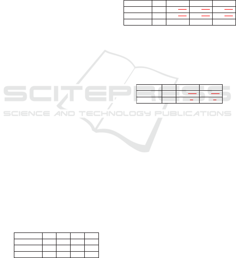
Table 2: The values in terms of S are adjusted in order to
compensate for the proposed change on P.
A B C D
P (1000 $) 110 110 120 110 115 110 160
S (m
2
) 115 120 130 118 125 115 145
D
ist
(km) 4 4,5 3 2
Now that all four alternatives have the same value on
P, P is cancelled out as irrelevant. Furthermore, A
is dominated by D and is eliminated. X proceeds by
choosing S as the referencecriterion and D
ist
as the re-
sponse criterion. The result after making adjustments
is given in table 3.
Table 3: The values in terms of D
ist
are adjusted in order to
compensate for the proposed change on S.
B C D
S (m
2
) 120 120 118 120 115
D
ist
(km) 4,5 3,5 3 2,8 2
As S is now cancelled out as irrelevant, alternative D
is chosen as the best alternative with the value of 2,8
in terms of D
ist
(the only remaining criterion).
3.2 GISwaps
The Even Swaps method, as presented in Section 3.1,
is only suitable for decision-making in discrete choice
models, when the number of alternatives is relatively
small. Many GIS-related decision-making situations
concern a continuous choice model, where the num-
ber of alternatives is only constrained by the limits
of the used data representation model. For example,
finding the optimal location for a certain purpose in
an area represented by a 1000 x 1000 grid, the num-
ber of alternatives could be as high as 1 000 000, de-
pending on the grid resolution and specific constraints
of the problem. If the mechanism of the Even Swaps
method is to be applied to geospatial problems, the
process of making trade-offsneeds to be automatized.
For this purpose we introduce GISwaps, an approach
that makes decision making based on even swaps in
decision problems with large number of alternatives
manageable. The method, which is described in de-
tail in Milutinovic et al. (2017), uses input from the
IVAPP 2018 - International Conference on Information Visualization Theory and Applications
238

decision maker on a number of virtual alternatives in
order to calculate, for each alternative in the set, the
coefficient of the value change (swap coefficient) on
the response criterion. As the name suggests, the vir-
tual alternativesdo not need to actually exist in the set,
but are hypothetical alternatives used to fine-tune the
value update function. The number of virtual alterna-
tives, as well as assigned descriptive values in terms
of each criterion, are set in each step for the current
reference and response criteria, respectively.
Unlike Even Swaps, GISwaps does not incorpo-
rate elimination of dominated alternatives. In geospa-
tial decision making we usually want to obtain an or-
dered set of all feasible alternatives, as opposed to a
single best alternative. In its basic form, our method
can be expressed by the following algorithm:
Repeat
Decide the reference criterion R
Decide the response criterion M
Set virtual alternatives
Obtain trade-off values for virtual alternatives
Calculate update coefficients for virtual alternatives
For each alternative in the set
Calculate the update coefficient for the alternative
Update the value of the alternative with respect to M
Discard R
Until a single criterion remains
Rank the alternatives
In a typical geospatial site location problem, a
number of possibly conflicting criteria is usually con-
sidered. Finding the optimal site location for building
a dam, for example, requires considering factors such
as water discharge, undulation, hydraulic head, dis-
tance to urban areas, distance to forests and distance
to agricultural areas. Applying GISwaps on such case
would take five swap turns, one of the criteria being
cancelled out in each turn. In the following example,
we explain our method on one possible turn, where
hydraulic head is used as the reference, and undula-
tion as the response criterion. We use 16 virtual alter-
natives in order to fine-tune the value update function.
Each of the alternatives is assigned a pair of values: a
value from the arrayV
R
(four reference values in terms
of the reference criterion R) and a value from the array
V
M
(four reference values in terms of the response cri-
terion M). We use following reference values for the
virtual alternatives in terms of R and M, respectively:
V
R
= [R
min
,R
min
+ R
q
,R
min
+ 2R
q
,R
min
+ 3R
q
]
V
M
= [M
min
+ M
q
,M
min
+ 2M
q
,M
min
+ 3M
q
,M
max
]
(1)
where
R
min
: minimum value with respect to R
R
max
: maximum value with respect to R
R
q
= (R
max
− R
min
)/4
M
min
: minimum value with respect to M
M
max
: maximum value with respect to M
M
q
= (M
max
− M
min
)/4
For example, for hydraulic head values in range 1-
46 and undulation values in range 1-136, it gives the
following values for V
R
and V
M
, respectively:
V
R
= [1,12.3,23.5,34.8]
V
M
= [35,68,103,136]
(2)
Based on his/her judgement and preferences, the deci-
sion maker now needs to perform even swaps. He/she
chooses a compensation value M
u
(i, j)
of criterion M
for each virtual alternative, i.e. for each pair of ref-
erence values (V
R
(i)
,V
M
( j)
); i, j ∈ [1..4]. Each value
M
u
(i, j)
is chosen so that the decision maker is in-
different between the differences (R
max
− V
R
(i)
) and
(V
M
( j)
− M
u
(i, j)
). The compensation values are stored
in a 4x4 matrix M
u
(Equation 3). With the input from
the decision maker as shown in Figure 1, the M
u
ma-
trix contains following values:
M
u
=
18 40 57 87
20 44 66 91
22 50 70 95
28 59 84 106
(3)
Update coefficients for each element in M
u
are stored
in corresponding matrix M
c
. Each value M
c
(i, j)
is cal-
culated as
M
c
(i, j)
=
V
M
( j)
− M
u
(i, j)
R
max
− V
R
(i)
(4)
For the input used in the example, the M
c
matrix con-
tains following values:
M
c
=
0.37 0.63 1.01 1.09
0.44 0.73 1.08 1.33
0.57 0.82 1.44 1.82
0.60 0.85 1.66 2.69
(5)
In order to calculate the update coefficient for an al-
ternativea, we need to determine index i using a
R
(the
value of a in terms of the reference criterion R) and in-
dex j using a
M
(the value of a in terms of the response
criterion M). The indexes are determined as follows:
i = k for V
R
[k]
≤ a
R
< V
R
[k+1]
, k ∈ [1..3]
i = 4 for a
R
≥ V
R
[4]
j = 1 for a
M
≤ V
M
[1]
j = k for V
M
[k−1]
< a
M
≤ V
M
[k]
, k ∈ [2..4]
(6)
The value update coefficient for any alternative a can
now be calculated as
a
c
= M
c
(i, j−1)
+
(M
c
(i, j)
− M
c
(i, j−1)
) ·
a
M
− V
M
( j−1)
V
M
( j)
− V
M
( j−1)
(7)
Visual GISwaps - An Interactive Visualization Framework for Geospatial Decision Making
239

The remaining four turns are performed in the same
manner. After cancelling out five of six criteria, the
grid containing the values for the only remaining cri-
terion would be the de facto result of the decision pro-
cess that can be shown in an appropriate GIS soft-
ware.
While GISwaps enables interactive definition of
compensation values and a fully automatized up-
date of response criteria in a quasi-continuous multi-
criteria decision model, it requires suitable visualiza-
tions of the outcomes in the iterative process of up-
dating coefficients and elimination of reference crite-
ria. In the following section we present our approach
to visualizing the complex relationships between the
choice of reference and response criteria, the design
of the update coefficients, and their effect on the huge
amount of alternatives both in attribute space and ge-
ographical space.
4 VISUAL GISwaps
The GISwaps method is an interactive method for
spatial decision making. Through a semi-automatized
process explained in Section 3.2, the decision maker
sets the actual trade-off values between alternatives
with respect to a pair of criteria. Throughout the pro-
cess, the decision maker is active and in full control.
The interactive visualization presented in this sec-
tion allows the decision maker to explore the conse-
quences of trade-offs and costs accepted during each
step of the iterative decision process.
The main window of the application that imple-
ments the GISwaps method as well as the visualiza-
tion framework is given in Figure 1. The image shows
the setup of the example used in Section 3.2, after the
decision maker has selected reference (in the appli-
cation referred to as measuring stick) and response
criteria, and set compensation values in terms of the
latter. The example is used in this section with the
same trade-off values as in Section 3.2.
Our interactive visualization frameworkintegrates
fundamental visualization techniques, and consists of
three conceptual units: 1) visualization of alterna-
tives in attribute space, 2) visualization of alternatives
in geographical space, and 3) visualization of value
functions. In each step of the iterative process, ref-
erence and response criteria are selected by the deci-
sion maker. The scatterplot representing the attribute
space for the set of alternatives is constructed as a
2D-plot, with position on the X-axis determined by
the value in terms of the response criterion, and po-
sition on the Y-axis determined by the value in terms
of the reference criterion. This representation gives
the decision maker an insight into the distribution of
data in terms of the currently chosen response crite-
rion. An extra dimension may be added to the plot by
color-coding samples in order to show values of the
alternatives in terms of a third criterion, that we will
refer to as comparison criterion. Even though the val-
ues of the alternatives in terms of the comparison cri-
terion are not changed, and the comparison criterion
should not be directly considered when determining
trade-off values for the response criterion in the cur-
rent iteration, this extra information gives the deci-
sion maker a deeper insight and better understanding
of the consequences of the performed trade-offs. The
comparison criterion is chosen by the decision maker
from the list of non-cancelled criteria. An example of
a non-color-coded and a color-coded plot is given in
Figure 2. The positions of the alternatives are updated
and the plot redrawn each time the decision maker
changes a value in terms of the response criterion of
any of the virtual alternatives. In order for the deci-
sion maker to be able to explore and make judgements
regarding the consequences of a change, the original
positions of alternatives are shown in the plot in light
blue color. This gives the decision maker a better un-
derstanding of not only the magnitude of change re-
sulting from the proposed trade-off values, but even
the distribution of change, i.e. how many alternatives
are affected by the proposed trade-off. By clicking
on and highlighting a point in the plot, the decision
maker gains access to further information about the
selected alternative. A vector representing the magni-
tude of change in terms of the response criterion af-
ter the suggested trade-off is shown in the plot as the
distance between the original and current value (po-
sition), as a complement to the numeric information.
Furthermore, the selected alternative is highlighted in
the map panel, giving the decision maker information
about the position of the alternative in the geographi-
cal space. An example is shown in Figure 3. The part
of the visualization that concerns geographical space
consists of two maps of the geographic area where the
decision problem is situated. The two maps simulta-
neously show color-coding for both response criterion
and comparison criterion (if any). The geographic
distribution of the alternatives in the left map is al-
ways color-coded by values of alternatives in terms of
the response criterion. The color-coding in the right
map is related to the color-coding in the scatterplot,
i.e. it shows the values of the alternatives in terms of
the comparison criterion if there is one selected, and
is not color-coded otherwise. In Figure 3, Discharge
was chosen as comparison criterion.
Visualization of value functions is given in form
of a multi-line chart, with the number of lines de-
IVAPP 2018 - International Conference on Information Visualization Theory and Applications
240
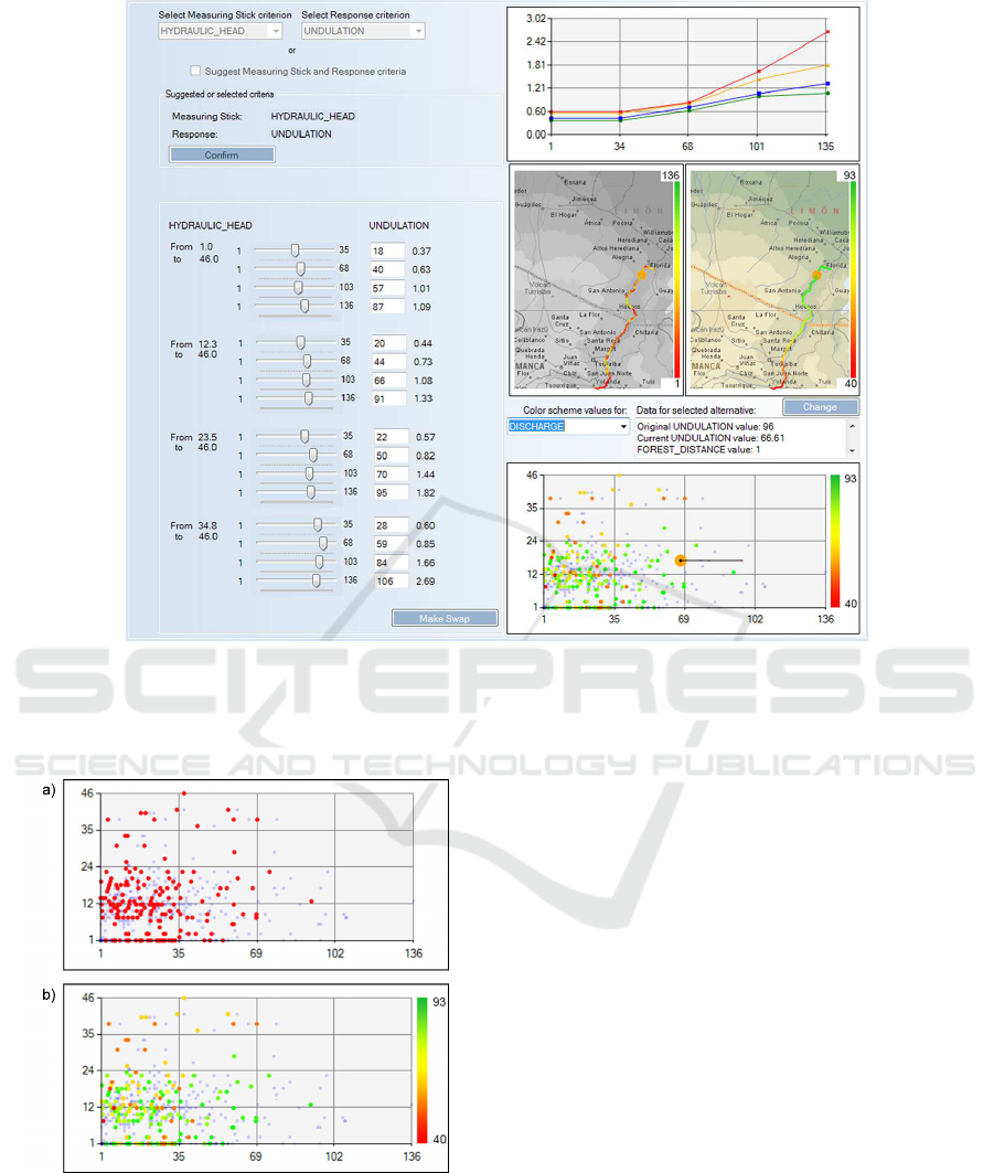
Figure 1: Main window of the application implementing GISwaps and the visualization framework. Adjusting the values in
terms of the response criterion (Undulation, in the example), in order to compensate for the changes made in the reference
criterion (Hydraulic head), is performed in the left panel. The right panel contains attribute space visualization scatterplot
(bottom), geographical space visualization maps (middle), and value functions visualization (top).
Figure 2: Scatterplot for the example decision problem with
no comparison criterion selected (a) and with Discharge se-
lected as the comparison criterion (b).
termined by the number of elements in V
R
and the
number of points defining each line determined by the
number of elements in V
M
(see Equation 1 in Section
3.2). An example is given in Figure 4. This visual
representation makes potential deviations in a value
function evident, allowing the decision maker to ad-
just suggested values if the deviationis due to an error,
rather than personal preference and judgement.
5 DISCUSSION AND
CONCLUSIONS
In Keeney and Raiffa (1976), the essence of the is-
sue of trade-offs under certainty is described as “How
much achievement on objective 1 is the decision
maker willing to give up in order to improve achieve-
ment on objective 2 by some fixed amount?”. As the
authors point out, the trade-off issue usually requires
subjective judgement of the decision maker. As a
trade-off method based on even swaps, GISwaps is
an intuitive and efficient tool capable to address one
of the big challenges in the context of decision sup-
port systems, namely, how to handle the preferences
of the decision maker. Instead of being concerned
with the abstract concept of the relative importance of
decision criteria, using GISwaps the decision maker
Visual GISwaps - An Interactive Visualization Framework for Geospatial Decision Making
241
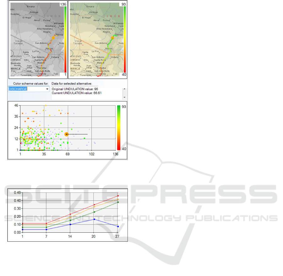
Figure 3: When an alternative is selected, its magnitude of
change is shown, as well as its position in the geographical
space (highlighted in the map panel).
Figure 4: Visualization of value functions. The number of
functions (lines) is determined by the number of elements
in V
R
.
works with concrete values and differences, which we
believemakes our method more flexible than the com-
monly used approach of combining weighting and ag-
gregation methods.
Geospatial multi-criteria decision problems tend
to be complex, with a large number of conflicting cri-
teria to be taken into consideration, and thousands or
even millions of alternatives to be evaluated and com-
pared. In order for the decision maker to have a good
understanding of the consequences of his/her choices,
numeric data needs to be complemented by a visual
representation of relevant information that would be
unavailable otherwise. In an interactive decision-
making method, this needs to be done at each step
of the decision-making process.
The positiveimpact of the interactivevisualization
presented in this paper is multifaceted:
• The scatterplot representation of the alternatives
in the attribute space gives the decision maker an
insight into the distribution of data in terms of the
currently chosen response criterion. From Figure
2, for example, it is obviousthat only a small num-
ber of alternatives has the undulation value in the
upper half of the range, i.e. over 68.
• It reveals potential outliers. Outliers, both posi-
tive and negative, may have a significant impact
on the reliability of the values interpolated from
the values assigned to virtual alternatives; for that
reason, they should not pass unnoticed.
• It gives the decision maker the possibility to get
a closer look at the alternatives of interest. Ex-
tra information available on demand includes the
original value, the current value and the magni-
tude of change in terms of the response criteria,
the value of the alternative in terms of any of the
non-cancelled criteria, and the geographic loca-
tion of the alternative. This information is of great
importance for understanding the impact of a sug-
gested trade-off.
• The map view helps the decision maker make
more sensitive choices. By being able to see the
geographic location of the selected alternative, the
decision maker can, based on his/her knowledge
and preferences, re-evaluate suggested trade-offs
that would affect the alternative(s) of interest.
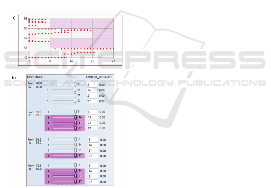
• Our visualization saves the decision maker time
and effort. The prime assumption for any trade-
off based method for decision making to be suc-
cessful is that the trade-offs are balanced and care-
fully performed. Deciding trade-offvaluesfor vir-
tual alternatives that might not have any impact on
the outcome of the decision process is therefore
better avoided. By means of visual representation
of alternatives in the attribute space, the decision
maker can see if there are empty value intervals,
i.e. value ranges with no alternatives. In the ex-
ample in Figure 5, there are seven intervals out
of sixteen with no alternatives. Consequently, it
is unnecessary to decide trade-off values for the
virtual alternatives that define those intervals.
• It helps the decision maker make consistent trade-
offs. The significance of the value functions
chart increases with the number of virtual alter-
natives. In many cases, the decision maker wants
the trade-off values to be consistent over the set of
virtual alternatives. Making consistent trade-offs
based on numeric values only is a demanding task,
and the complexity of the task increases with the
number of virtual alternatives. Visual representa-
tion makes potential deviations in a value function
IVAPP 2018 - International Conference on Information Visualization Theory and Applications
242
evident (see Figure 4; the function represented by
the blue line shows a deviation for x = 27), allow-
ing the decision maker to adjust suggested values
if the deviation is due to an error, rather than per-
sonal preference and judgement.
The GISwaps method and the interactive visualiza-
tion presented here are designed and developed in
close cooperation with experts in multi-criteria deci-
sion making and geographic information systems. At
this point, though, they have not been used by practi-
tioners in the field of GIS-MCDM. In a forthcoming
study, the GISwaps method will be evaluated with re-
spect to efficiency and usability, in comparison with
the combination of AHP and the weighted summation
method, which is the most commonly used approach
in geospatial decision-making. Based on the results,
a second study will be carried out, where the impact
of the interactive visualization framework presented
in this paper will be evaluated.
Figure 5: a) Empty intervals, i.e. intervals that contain no
alternatives; b) Virtual alternatives for which it is unneces-
sary to set trade-off values, as they define empty intervals.
REFERENCES
Andrienko, N. and Andrienko, G. (2003). Informed spa-
tial decisions through coordinated views. Information
Visualization, 2(4):270–285.
Andrienko, N. and Andrienko, G. (2004). Interactive visual
tools to explore spatio-temporal variation. Proceed-
ings of the working conference on Advanced visual
interfaces - AVI ’04, page 417.
Andrienko, N., Andrienko, G., and Gatalsky, P. (2003). Ex-
ploratory spatio-temporal visualization: An analytical
review. Journal of Visual Languages and Computing,
14(6):503–541.
Bautista, J. and Carenini, G. (2006). An integrated task-
based framework for the design and evaluation of vi-
sualizations to support preferential choice. Proceed-
ings of the working conference on Advanced visual in-
terfaces - AVI ’06, (February):217.
Carenini, G. and Loyd, J. (2004). Valuecharts: Analyzing
linear models expressing preferences and evaluations.
Proceedings of the working conference on Advanced
visual interfaces - AVI ’04, (February):150.
Chrisman, N. R. (1999). What does ’gis’ mean? Transac-
tions in GIS, 3(2):175–186.
Cowen, D. (1988). Gis versus cad versus dbms: what are the
differences. Photogrammetric Engineering and Re-
mote Sensing, (54):1551–1555.
Hammond, J. S., Keeney, R. L., and Raiffa, H. (1998). Even
swaps: A rational method for making trade-offs. Har-
vard Business Review, 76(2):137–149.
Hammond, J. S., Keeney, R. L., and Raiffa, H. (1999).
Smart Choices - a practical guide to making better
life decisions. Broadway Books, New York, USA, 1st
edition.
Jankowski, P., Andrienko, N., and Andrienko, G. (2001).
Map-centred exploratory approach to multiple criteria
spatial decision making. International Journal of Ge-
ographical Information Science, 15(2):101–127.
Keeney, R. L. and Raiffa, H. (1976). Decisions with Multi-
ple Objectives - Preferences and Value Tradeoffs. John
Wiley & Sons, Inc., USA.
Kollat, J. B. and Reed, P. (2007). A framework for visually
interactive decision-making and design using evolu-
tionary multi-objective optimization (video). Environ-
mental Modelling and Software, 22(12):1691–1704.
Li, H. L. and Ma, L. C. (2008). Visualizing decision process
on spheres based on the even swap concept. Decision
Support Systems, 45(2):354–367.
Malczewski, J. and Rinner, C. (2015). Multicriteria De-
cision Analysis in Geographic Information Science.
Springer, New York, USA.
Miettinen, K. (2014). Survey of methods to visualize alter-
natives in multiple criteria decision making problems.
OR Spectrum, 36(1):3–37.
Milutinovic, G., Ahonen-Jonnart, U., and Seipel, S. (2017).
Giswaps - a new method for decision making in
continuous choice models based on even swaps.
Manuscript submitted for publication.
Simon, H. A. (1960). New science of management decision.
Harper, New York, USA.
Visual GISwaps - An Interactive Visualization Framework for Geospatial Decision Making
243
