
A Visual Analytics Framework for Exploring Uncertainties in Reservoir
Models
Zahra Sahaf
1
, Hamidreza Hamdi
1,2
, Roberta Cabral Ramos Mota
1
, Mario Costa Sousa
1
and Frank Maurer
1
1
Department of Computer Science, University of Calgary, Calgary, Canada
2
Department of Geoscience, University of Calgary, Calgary, Canada
Keywords:
Visual Analytics, Mutual Information, Clustering, Uncertainty Analysis, Volumetric Ensembles.
Abstract:
Geological uncertainty is an essential element that affects the prediction of hydrocarbon production. The
standard approach to address the geological uncertainty is to generate a large number of random 3D geological
models and then perform flow simulations for each of them. Such a brute-force approach is not efficient as
the flow simulations are computationally costly and as a result, domain experts cannot afford running a large
number of simulations. Therefore, it is critically important to be able to address the uncertainty using a few
geological models, which can reasonably represent the overall uncertainty of the ensemble. Our goal is to
design and develop a visual analytics framework to filter the geological models and to only select models
that can potentially cover the uncertain space. This framework is based on the mutual information for the
calculation of the distance between the models and clustering for the grouping of similar models. Interactive
visualization tasks have also been designed to make the whole process more understandable. Finally, we
evaluated our results by comparing with the existent brute force approach.
1 INTRODUCTION
Uncertainty is related to poor knowledge of a phe-
nomenon. In petroleum engineering applications, for
instance, we have lots of uncertainties in all aspects
of petroleum production phases. This is essentially
due to a large number of unknows that exist at any
particular stage of exploration, development, and pro-
duction workflow. In the exploration phase, which
is the focus of this paper, the lack of knowledge in
representing the measured data (e.g., due to noise),
expressing the depositional settings, spatial configu-
rations of the rock types, or mathematical uncertainty
in representing the geology, are the key elements that
largely impact the decision making process based on
modeling (Caers, 2011).
Reservoir models are essential to portray the im-
pact of uncertainty. A reservoir model is a 3D grid-
based digital representation model of the subsurface
composed of a large number of cells/voxels. Each
cell has a location in space and a set of attributes de-
scribing geological properties (such as porosity and
permeability).
Geostatistical methods are used to estimate at-
tribute values of the cells where no information is
available. The inherent uncertainties of these geosta-
tistical models imply that the attribute values of a cell
can be assigned to different values and still be consis-
tent with known facts. Geologists capture the inher-
ent uncertainty by creating a large number of models.
Flow simulations then take the models as an input and
determine the expected outcome on variables of inter-
est (like overall oil production volume) over time. The
large number of cells in the digital reservoir model
and the computational cost of processing flow simu-
lations (i.e., usually requiring several hours) prohibit
a brute-force approach for conducting the numerical
flow simulation for all possible models. Therefore,
it is substantially favorable to carefully select a few
models with great diversity that can reasonably repre-
sent the overall uncertainty (Idrobo et al., 2000).
Another critical requirement for domain experts is
an efficient way to compare the 3D models in a large
ensemble without running the costly flow simulations.
This aspect can help identify how models are different
or similar to each other spatially and visually. Using
that, the users can find out which spatial areas have
more contribution toward quantifying the uncertainty
and thereby the oil production.
To address all these requirements, we have de-
74
Sahaf, Z., Hamdi, H., Mota, R., Sousa, M. and Maurer, F.
A Visual Analytics Framework for Exploring Uncertainties in Reser voir Models.
DOI: 10.5220/0006608500740084
In Proceedings of the 13th International Joint Conference on Computer Vision, Imaging and Computer Graphics Theory and Applications (VISIGRAPP 2018) - Volume 3: IVAPP, pages 74-84
ISBN: 978-989-758-289-9
Copyright © 2018 by SCITEPRESS – Science and Technology Publications, Lda. All rights reserved

signed and developed a visual analytics framework
to identify the models that can potentially cover the
uncertain space (that is referred to as ”representative
models”). The proposed process can resolve exist-
ing issues of previous studies. Current techniques
like ranking (Ballin et al., 1992), random selection, or
probability-based techniques (Rahim and Li, 2015),
are all costly regarding computation. They are auto-
matic processes preventing the domain experts from
guiding the selection process. Moreover, they are not
modular and target only some specific types of reser-
voirs (Yazdi and Jensen, 2014).
The first step in the proposed process is to es-
tablish a representative metric for calculating the
(dis)similarity between a pair of 3D geological mod-
els. As such, a new distance measure has been de-
signed based on the mutual information (MI) concept
(Lin, 1998) (Goshtasby, 2012). Distances are then
employed within a clustering algorithm to create sets
of similar models (i.e., models where simulation re-
sults are likely to be similar). In this state, cluster cen-
ters are identified as the default representative mod-
els, and the users can only run the simulation for this
limited set of selected models. We show the accu-
racy of our selection method by comparing the actual
flow simulation results of the selected models with the
brute-force approach. A particular selection is accu-
rate when the simulation results of all models in one
cluster are very similar to each other. In addition, the
representative models should cover a similar cumula-
tive hydrocarbon production uncertainty range as the
brute force approach. In summary, the main contribu-
tions of this paper are:
• Novel dis(similarity) metric for calculating pair-
wise distances between the 3D geological models
(section 5).
• Analytical framework for uncertainty assessment
of dynamic properties (e.g. oil production) that
utilizes our proposed similarity metric (section 4
and 6).
• A visual analytics tool that supports the proposed
framework and provides visual and interactive
tasks for steering the uncertainty assessment pro-
cess (section 8).
2 RELATED WORK
2.1 Current Approaches for Selecting of
Geological Models
Various methods are available for selecting geologi-
cal realizations which can be broadly classified as ran-
dom selection, ranking, probability distance-based re-
alization reduction method, and clustering technique.
While randomly selecting a subset of realizations
is a straightforward method for implementation, it
may result in a wrong measure of geological uncer-
tainty especially when the number of selected real-
izations is small. Ranking (Ballin et al., 1992) is the
most common method for selecting geological real-
izations. This method arranges the geostatistical mod-
els based on an easily computable measure in an as-
cending/descending order and then selects the ones
that have low, medium, and high values of that mea-
surement. One of the major limitation of the existing
ranking methods is that they rely significantly on the
measure used. If the measure has a weak correlation
with the production of the reservoir, then the selected
models will not adequately represent the full set of
realizations (Li et al., 2012).
Probability distance-based realization reduc-
tion/selection methods have also been recently
investigated by some researchers (Rahim and Li,
2015). In this approach, an optimization problem
is solved to find an optimal subset that has similar
statistical distribution characteristics to the superset
of models. The main issue with these optimization
problems is that they could be very complicated and
time-consuming for a broad set of models, and in
the presence of the outlier models, the optimization
process might not converge. Clustering methods
have also been proposed recently in the domain. For
instance, (Scheidt and Caers, 2010) used simplified
simulation results to compute the distance between
the models to form a distance matrix. Then these
distances were used to perform the clustering. The
need of petroleum industry to address the geological
uncertainty using a limited number of geological
realizations necessitates designing an analytical
framework that is computationally less expensive,
dependent on the static properties of geological
models rather than flow simulation results, visual and
interactive, and capable of showing differences and
similarities between the models.
2.2 Visual Analytics Techniques for
Multirun Data
The most similar dataset in computer science domain
to the geological models in petroleum engineering is
multirun models. In areas such as climate research
and engineering, multirun data is often generated to
study the variability of models and to understand
the model sensitivity to specific control parameters
(Kehrer and Hauser, 2013). In general, multirun data
stem from a type of process (like geostatistical algo-
A Visual Analytics Framework for Exploring Uncertainties in Reservoir Models
75

rithms in our case) that is repeated multiple times with
varied parameter settings, leading to a large number
of collocated data volumes (Wilson and Potter, 2009).
Since multirun data consists of a superset of volumet-
ric models, their representation and analysis are chal-
lenging.
The representation of multirun data is somewhat
new to the visualization community. It is a challeng-
ing task since the data is often high dimensional, mul-
tivariate, and large at the same time. Accordingly, one
of the common ways is to aggregate the distributions
of multirun data, by computing statistical summaries
(Love et al., 2005). Subsequently, the resulting data is
visualized using mainly box plots (Kao et al., 2002),
line charts (Demir et al., 2014), glyphs (Kehrer et al.,
2011), or InfoVis techniques such as parallel coordi-
nates or scatterplot matrices combined with statistics
(Nocke et al., 2007).
On the analytics side of multirun data, statisti-
cal methods are among the first candidates to be
used for reducing the data dimensionality. For ex-
ample, (Kehrer et al., 2010) proposes a method to
integrate statistical moments (mean, variance, skew-
ness, and kurtosis) into the visual analysis of multi-
run data. Alternatively, mathematical and procedural
operators are also used to transform the multirun data
into some compact forms (e.g., streamlines, isosur-
faces, or pseudocoloring) where existing visualization
techniques are applicable (Love et al., 2005) (Fofonov
et al., 2016).
Data mining techniques are also among the recent
methods being used to explore the multirun data (Cor-
rea et al., 2009). (Bordoloi et al., 2004) applied hi-
erarchal clustering techniques to multirun data. In
a recent work, Bruckner and Moller (Bruckner and
Moller, 2010) presented a result driven exploration
approach for physically-based multirun simulations.
Each volumetric time sequence is first split into sim-
ilar segments over time and then is grouped across
different runs using a density-based clustering algo-
rithm. This approach supports the user in identifying
similar behavior across different simulation runs.
Our analytics approach fits into the data min-
ing category since the similarity between ensembles
needs to be discovered both effectively and visually.
However, most of the proposed clustering approaches
are based on the 2D ensembles such as images. Even
though the 3D ensembles are available, their aggrega-
tions are used for the clustering task. In this work, we
want to perform the clustering on the 3D ensembles
directly without using their aggregation, and that re-
quires an accurate definition of distance between ge-
ological 3D ensembles.
3 REQUIREMENT ANALYSIS
Through extensive discussions with the reservoir en-
gineers from our industry partners, we gathered the
following required elements as engineering require-
ments needed for designing a useful analytics frame-
work:
R1. Limited selection of reservoir models. How
can we select few representative models from a super
set of models?
R2. Low computational cost. How can we have
a fast selection process? The reason is that reservoir
engineers usually want to save time in the engineering
tasks (running costly simulations) as much as possi-
ble.
R3. Flexibility on the reservoir properties used
in the selection process. Depending on the type of
reservoir, different reservoir properties are provided.
R4. Flexibility on the area of interest. How can
we perform the selection process based on an area of
interest in the reservoir model? Usually, only specific
areas of reservoir model (e.g., areas around wells) are
considered significant. Therefore, there is a need to
perform the selection process based on a region of in-
terest that the user selects.
R5. Illustration of reservoirs (dis)similarity dis-
tance. For instance, which area of models contribute
more in the (dis)similarity value or how to spatially
and visually observe the comparison between a set of
3D reservoir models.
4 ANALYTICAL FRAMEWORK
FOR DESCRIPTIVE
UNCERTAINTY ASSESSMENT:
OVERVIEW
An overview of our proposed process is represented
in Figure 1. Initially, we have a set of 3D geologi-
cal models (a). Our proposed block-based similarity
metric is calculated for all pairs of models (b). The
similarity values are then utilized to project models
into a 2D space using multidimensional scaling tech-
niques (c). Each point in 2D space corresponds to
a 3D model. The distance between points in the pro-
jected space represents the similarity between models,
the closer the points, the more similar the 3D mod-
els. The final step is to cluster the points and pick
a representative model from each cluster (d). The is
an iterative and interactive process, which depends on
the size of the similarity block, clustering property,
the number of clusters, etc. Each of these stages is
explained in more detail in the subsequent sections.
IVAPP 2018 - International Conference on Information Visualization Theory and Applications
76
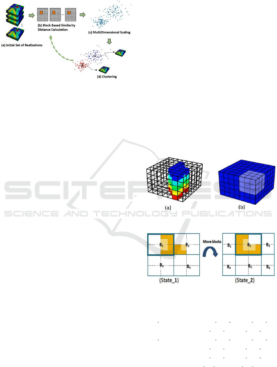
Figure 1: Overview of proposed filtering Process.
5 CALCULATION OF
(DIS)SIMILARITY METRIC
A majority of reservoir simulation studies are per-
formed on a single geological model. Therefore, ’dis-
tance’ between reservoir models is somewhat new
concept in that domain (Fenwick and Batycky, 2011).
Therefore it is essential to define a distance that re-
flects the requirement of the engineering tasks. Two
models are called similar when they have a sim-
ilar dynamic result (reservoir performance). The
(dis)similarity distance can be calculated in a manner
that should leverage two primary requirements. First,
it has to be well correlated to the dynamic behav-
ior of reservoir or flow response(s) interest (Scheidt
et al., 2009). Second, its calculation should not be
very costly. According to our discussions with the
domain experts and domain literature evaluation stud-
ies (Rahim and Li, 2015), static measures meet the
two mentioned requirements and much preferred than
dynamic measures. The reason is that static mea-
sures are simplified metrics designed to achieve a
good correlation with the reservoir production perfor-
mance variable of interest. For instance, Original oil-
in-place(OOIP) is one of the critical terms calculated
in reservoir simulation. It is calculated by the sum-
mation of the product of the following static proper-
ties volume (V), porosity (φ) and oil saturation of cell
c (OOIP =
∑
c
(V
c
φ
c
(1 − S
c
))). Therefore, it shows
how static properties are highly correlated with the
dynamic (flow) terms. In addition to that, static mea-
sures are computationally much easier for evaluation
when compared to reservoir flow simulation. It can
be easily calculated for a broad set of realization (R2).
In the next sections, we explain how these static mea-
sures use with our proposed similarity metric.
Reservoir models have 3D geometries with corre-
lated spatial properties. Additionally, they can have
some favorable 3D sub-structures (e.g., geological
channels). Hence, any appropriate similarity mea-
surement should be able to acknowledge these lat-
eral geological heterogeneities (Figure 2). Therefore,
we use a moving 3D template (block) approach to
calculate (dis)similarity distance between a pair of
models. The idea is to divide each 3D model into
a set of smaller 3D blocks (Figure 2) where each
block consists of a specific number of grid cells. The
(dis)similarity measure is computed between corre-
sponding blocks (templates) initially. Next, we take
an average of the(dis)similarity values between all
corresponding blocks. During this process, to reduce
the bias of the fixed spatial position of blocks, we
move the blocks in specific directions (x, y, z and di-
agonal) and distances (>1 and <block size). The fi-
nal distance will be the average of (dis)similarity val-
ues in all the possible movements. For simplicity, a
2D representation of movement is shown in Figure 3.
The yellow highlighted cells represent a prominent
geological feature. Equation 2 shows how the final
(dis)similarity is calculated between the two sample
models with one movement and two states.
Figure 2: (a) A sample important 3D structure in the geo-
logical models. (b) A sample 3D block.
Figure 3: Representation of a sample favorable structure
(highlighted in yellow), and movement of templates (dark
blue frames).
MI = MutualIn f ormation, Sim = Similarity, B = Block, M = Model (1)
(state 1)Sim(M1, M2) = mean(MI(M1 B1, M2 B1), MI(M1 B2, M2 B2),
MI(M1 B3, M2 B3), MI(M1 B4, M 2 B4))
(state 2)Sim(M1, M2) = mean(MI(M1 B1, M2 B1), MI(M1 B2, M2 B2),
MI(M1 B3, M2 B3), MI(M1 B4, M 2 B4),
MI(M1 B5, M2 B5), MI(M1 B6, M 2 B6))
TotalSim = mean(Sim(M1, M2) state 1, Sim(M1, M2) state 2)
Clearly, the similarity metric defined above can be
used for any geological property (R3). This can be
A Visual Analytics Framework for Exploring Uncertainties in Reservoir Models
77

specified interactively from the application interface
based on domain expert knowledge. There are also
scenarios that users need to consider multiple proper-
ties. In this scenario, (dis)similarity values are calcu-
lated separately for each property (using the proposed
approach) initially. After then, all those values are av-
eraged to determine the final (dis)similarity between
two models.
5.1 Distance Specification
The next step in the similarity calculation process is
to determine the distance between a pair of corre-
sponding 3D blocks. Similarity-based approaches are
widely used in different problems of science and en-
gineering. A number of distance-based formulations
have been proposed (Goshtasby, 2012), where Haus-
dorff and Euclidean distances are the most commonly
used in the reservoir engineering domain. The lat-
ter one is being found effective more for images and
2D surfaces such as time lapse seismic maps (Hut-
tenlocher et al., 1993), and Euclidean distance mostly
takes care of linear correlations. Therefore, we pro-
pose to use Mutual Information (MI) as a relatively
multi-purpose measure. MI is a popular information-
theoretic measure of similarity which has been ap-
plied in many areas of visualization and graphics do-
main like image registration, multi-modality fusion
and viewpoint selection (Bruckner and M
¨
oller, 2010)
(Haidacher et al., 2008). The major benefits of MI for
our case are:
1) Applicability. It is applicable as long as the do-
main has a probabilistic model. This aspect allows the
measure to be used in the domains where no similarity
measure has previously been proposed (e.g., reservoir
engineering domain).
2) Non-linear dependency detection. MI considers
all types of dependencies (i.e., linear and non-linear)
between two objects (Cover and Thomas, 2012). The
relationship between the property values in a pair of
geological models could be non-linear, and MI con-
siders all these types of dependencies.
3) Noise detection. Many studies show that MI is
robust to alleviate the impact of noise than the other
distances (Cole-Rhodes et al., 2003). Reservoir mod-
eling procedures can create outliers in the simulated
spatial structures. Therefore, it is critical not to be
sensitive to the noise data.
To further observe the effectiveness of MI over
other common distances in the domain, we create a
simplified dataset as represented in Figure 4. This
dataset can mimic some simplified channelized reser-
voir models. The first column (Figures 1, 4, 7) shows
the original models, some noise is added to the mod-
els in the second column (Figures 2, 5, 8), and the
models in the third column (Figures 3, 6, 9) are 90
degrees rotated. A reasonable distance should be less
sensitive to noise, in a way that the distance between
an original model and its noisy version should be min-
imal. On the other hand, the distance between an orig-
inal model and its rotated version should be consid-
erable, because they are indeed two different models.
Figure 5 shows the distance calculation for three met-
rics: MI, Euclidean, and Hausdorff distances. The re-
sults show that Euclidean distance is not sensitive to
rotation, and the Euclidean distance between a model
(1) and its rotated version (3) is zero, and they are
collocated in Figure 5. The similar pattern can be
seen for the other pair of models ((4,6) and (7,9)).
Although rotation is detected by Hausdorff distance
and the rotated models are located far from the origi-
nal models (see (1,4,7) vs (3,6,9) in Figure 5), noise
is not detected by this distance and noisy models are
considered as very different models and located far
from the original models ((see (1,4,7) vs (2,5,8) in
Figure 5). Finally, it can be seen how MI distance
detects movements like rotation and also ignores the
noise. For instance, models with their noisy version
are located close to each other such as (4,5), (1,2),
(7,8) in Figure 5. Moreover, on the other hand, move-
ments like rotation are also captured perfectly (see
how (6,3,9) in Figure 5 are located very far from the
original models). These benefits of MI can highlight
its effectiveness for many reservoir simulation stud-
ies. This is because, on one hand, even tiny move-
ments can translate to a significant effect on the sim-
ulation result, and on the other hand, modeling errors
can lead to creating some noisy structures in the geo-
logical models.
5.2 Block Size Specification
In this research, we advocate a block wise approach
for calculating the distance between the models. Such
a block-wise strategy is widely used in image and
video processing to exploit spatial and/or temporal
locality and coherence. A critical aspect of this ap-
proach is to select a proper block size. As sug-
gested by many researchers (Wang et al., 2008), block
size should not be too small to sacrifice performance.
Moreover, it should not be too large to ignore the lo-
cality and coherence feature of blocks. We use the
concept of entropy, as suggested in (Honarkhah and
Caers, 2010), to base the optimal block size. This op-
timal value is provided as a suggestion to the users in
our designed application; however, users can change
it based on their knowledge such as the use of corre-
lation length as it is used in generating some geolog-
IVAPP 2018 - International Conference on Information Visualization Theory and Applications
78
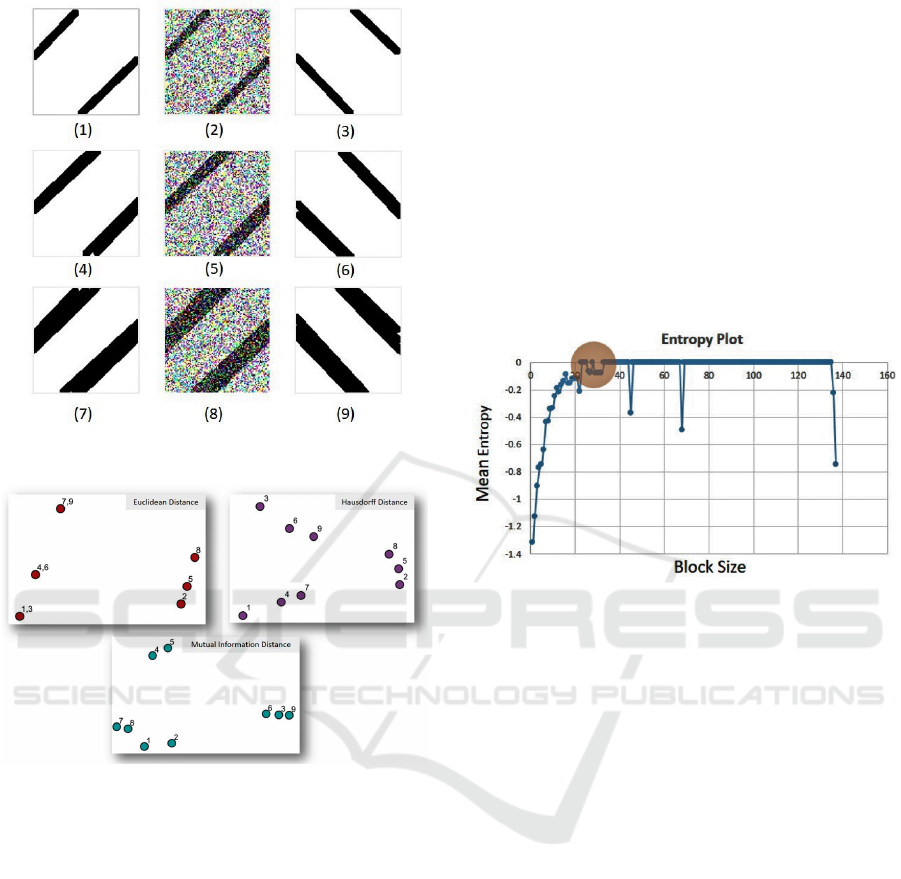
Figure 4: Dataset generated for evaluation of similarity dis-
tances.
Figure 5: Comparison of different distance calculation
methods including Euclidean, Hausdorff and Mutual Infor-
mation.
ical patterns. Entropy measures the information con-
tained in a message as opposed to the portion of the
message that is determined. This concept, when ap-
plied to blocks in reservoir models, can determine the
minimum information required to represent the whole
model reliably. Hence, our method for optimal block
selection is to scan a reservoir model with different
block sizes using our proposed moving block method.
For each block size, we calculate the average (mean)
entropy values of all blocks. Then, the entropy values
are plotted for each block size. We did some numeri-
cal experiments for this algorithm including using dif-
ferent reservoir models, blocks with different sizes in
each dimension, and blocks with equal sizes in all di-
mensions. Our empirical studies show the following
essential trends in the specification of block size:
• In the first stages of increasing block size, the en-
tropy sharply increases since the average number
of information bits needed to encode the underly-
ing patterns in the model is increasing.
• At a later stage where the block size has increased
above the optimal block size, entropy increases at
a much slower pace.
• In the stages that block size is close to the size of
the original model, entropy stops increasing. The
reason is that block contains repeated patterns and
hence, the amount of carried information ceases to
increase.
Therefore, according to these trends, the optimal size
of the block is in the stage that entropy slowly in-
creases as highlighted in Figure 6.
Figure 6: Mean entropy plot for different block sizes, with
highlighted maximum entropy.
Figure 6 shows the entropy plot for increasing the
block size (the scanning template) in the x direction.
The size of the original model in the x dimension is
140, and from Figure 6, it can be seen that a block size
with an x dimension around 25 to 30 (the highlighted
area) is an optimal value. This is where the average
entropy curve reaches its maximum for the first time.
We can perform a similar procedure for the y and z
dimensions, and get the optimal values for the other
dimensions as well. In our case, for a model with size
140 ×69 ×9, a block with size 23× 12 × 2 was found
to be the optimal size.
6 PROJECTION WITH
CLUSTERING
The calculated distances are utilized within a cluster-
ing algorithm to group similar models. Each clus-
ter center is a default representative member of the
containing cluster, which leads to our main require-
ment: to reduce the number of models needed for
simulation (R1). The K-Means clustering (KMC)
algorithm (Correa et al., 2009) is employed in this
step because of its computational efficiency on large
datasets. However, KMC suffers from a noticeable
A Visual Analytics Framework for Exploring Uncertainties in Reservoir Models
79
drawback. In the case where the data embeds a com-
plex structure (e.g., data are non-linearly separable),
a direct application of KMC is not suitable because
of its tendency to split data into globe-shaped clusters
(MacKay, 2003). To solve this problem, as suggested
in (Shawe-Taylor and Cristianini, 2004), data will be
mapped by a kernel transformation (Sch
¨
olkopf et al.,
1998) to a new space where samples become linearly
separable. Although there are many available kernel
functions in this study, we use radial basis function
(RBF). To make the RBF kernel more general - that
is not to be only the function of the Euclidean dis-
tance but also any other distances - the kernel is com-
bined with multidimensional scaling (MDS) (France
and Carroll, 2011) (Scheidt and Caers, 2010). MDS is
a classical approach that projects the original high di-
mensional space to a lower dimensional space, which
can preserve the original distances. In the projected
space, the spatial position is not critical; the crucial
aspect is the distance between projected points. The
closer points are to each other, the more similar they
are based on the initially defined distance. The pro-
jection algorithm is summarized as follows:
1. Use MI to calculate the block-based distance d(x
i
, x
j
) between each pair of models.
2. Use MDS to plot these locations in a low dimen-
sion, call these locations x
d,i
and x
d, j
with d the
dimension in the MDS plot.
3. Calculate the Euclidean distance between x
d,i
and
x
d, j
.
4. Calculate the kernel function with given σ .
K
i j
= K(x
i
, x
j
) = exp(
(x
d,i
− x
d, j
)
T
(x
d,i
− x
d, j
)
2σ
2
) (2)
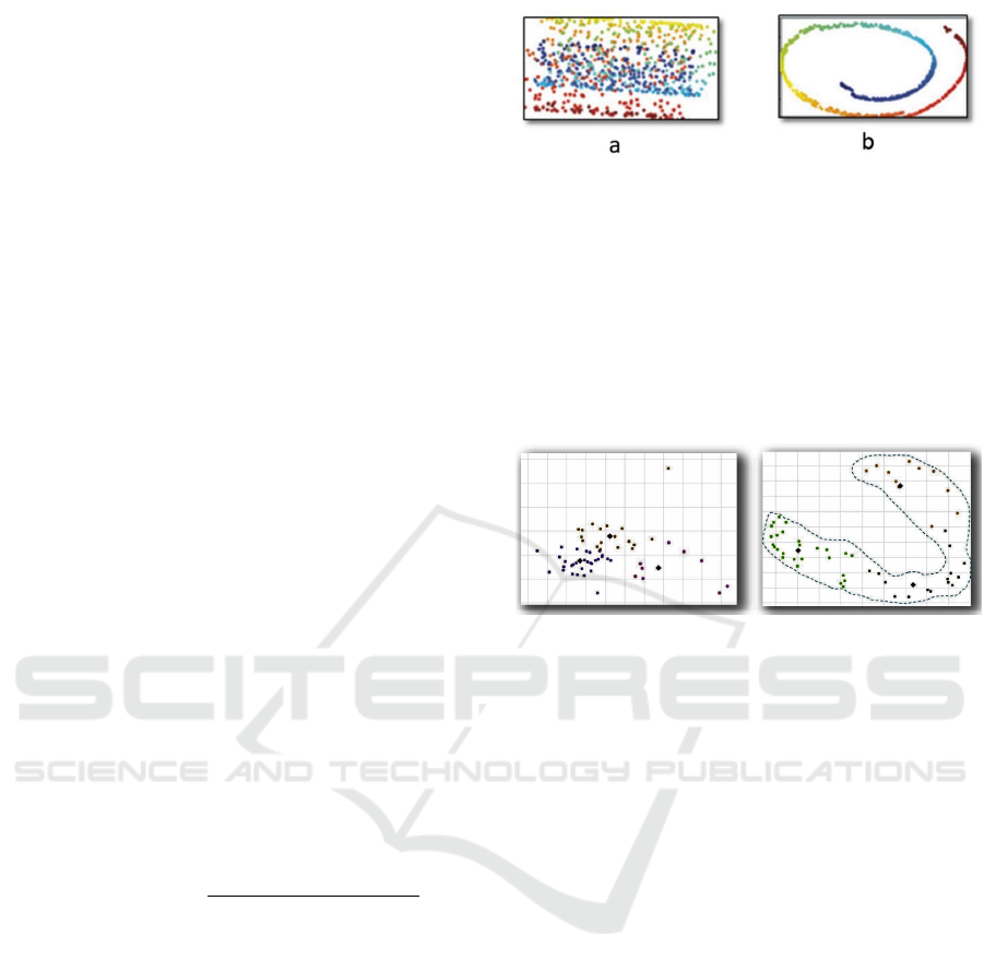
Other than having better and simpler visualiza-
tion of projected models using kernel transformation,
it has also a great benefit for clustering algorithm
(Scholkopf and Smola, 2001). K-means clustering
works well for cases such as Figure 7.b, but goes
wrong in complex cases such as Figure 7.a, where the
variation of objects/points in the 2D plot is nonlinear.
Therefore, it is frequently helpful to first transform
the points using a kernel transformation, as shown
in Figure 7.b, and then perform k-means clustering.
This technique is called kernel k-means in the litera-
ture (Williams, 2002) (Dhillon et al., 2004).
The efficiency of kernel KMC in clustering the ge-
ological models is shown in Figure 8. It shows how
the representation of data and clustering is different
in two scenarios: projection with and without kernel
transformation. It can be seen that the representation
of data looks better and more importantly clustering
Figure 7: (a) represents projection with MDS, (b) repre-
sents projection with MDS using kernel methods. (Zhang
et al., 2010).
results are more representative when a kernel transfor-
mation has been applied. Without kernel transforma-
tion, projected points are very close to each other, and
that makes separation of clusters complicated. How-
ever, with kernel transformation, a well organized and
linear structure can be seen in the results, and clusters
are better represented and separated.
Figure 8: Difference between multidimensional scaling
with (right) and without (left) kernel transformation on the
case study dataset.
7 EVALUATION
For evaluation of our proposed analytical framework,
we compared our results with the current alternative
process in the industry (i.e., to run flow simulation for
all models individually). We run the complete flow
simulation for all the models using the CMG reser-
voir simulator package, and plot the simulation re-
sults for the ’oil recovery factor’ dynamic property
(Figure 10). The plotted results show a range of un-
certainty on the oil production and we expect that our
cluster centers cover this range adequately. Regard-
ing the datasets, our industry partner generated differ-
ent datasets for us using different geostatistical algo-
rithms and scenarios. The idea was to cover almost
all different types of datasets in the domain. To evalu-
ate the performance of our proposed analytical frame-
work, they provided a various dataset with a different
number of Cartesian models (15 to 100 models) and
sizes (1000 to 100,000 cells). Therefore, we evalu-
ated our process in all different scenarios. In the first
simple scenario, 15 models were created in 5 groups,
and they only changed ’facies’ property in each group
(Figure 9). Facies is an important geological property
that reflects the rock type depositions. When we run
IVAPP 2018 - International Conference on Information Visualization Theory and Applications
80
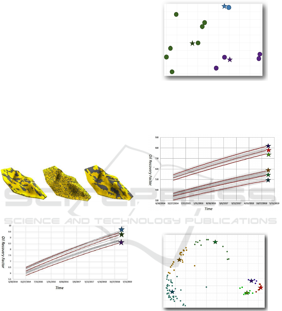
the flow simulation for all the 15 models, and plot a
dynamic property (like oil recovery factor vs time), a
range of uncertainty can be seen in the plotted curves
(high, medium and low recovery factor). To capture
this range of uncertainty with fewer of models, our
proposed filtering framework is used to cluster mod-
els into three clusters. Cluster centers are shown with
a star in Figure 11. The results show how cluster
centers can represent the range of uncertainty. High-
lighted curves in Figure 10 shows the cluster centers.
In addition to that, our approach is much faster than
the traditional brute-force approach. Depending on
the complexity and size of the reservoir model, the ex-
ecution time of a flow simulation could be different.
In this case study, running a complete flow simulation
takes around 5 minutes per model, that resulting in 75
minutes (an hour and a half) for all the models in total.
However, our approach takes around only 3 minutes
to calculate the distance between the models and gen-
erates the clustering result. Therefore, it can be seen
that our approach is very time efficient in comparison
to the existent techniques.
Figure 9: Different types of facies property that used for
the creation of geological models.
Figure 10: Simulation results of 15 geological models for
Oil Recovery Factor property.
In another scenario, domain experts changed the
value of all the properties (porosity, permeability, sat-
uration, etc) and they created 100 models. The idea
is to see how our proposed analytical framework per-
forms for such scenarios. Figure 12 shows the flow
simulation curves for all the 100 models. The range
of uncertainty is much broader than the previous sce-
nario. Our clustering result shows how this range
of uncertainty can be represented by only six models
(see the cluster center stars in Figure 13 and their cor-
responding curves in Figure 12). Similar to the pre-
vious case study, our approach had a very significant
Figure 11: Clustering result for 15 geological models.
performance in comparison to the current brute force
approach. The reason is that the flow simulations for
all the 100 models took around 7 hours, while our ap-
proach generates the clustering results in only 45 min-
utes.
Figure 12: Simulation results of 100 geological models for
Oil Recovery Factor.
Figure 13: Clustering result for 100 geological models.
8 VISUAL ANALYTICS
APPLICATION
This selection process has been designed and devel-
oped in a visual analytics framework (Figure 14). It
helps the users perform the selection process with a
set of user-defined parameters and compare the mod-
els at different levels of details and views. The users
A Visual Analytics Framework for Exploring Uncertainties in Reservoir Models
81
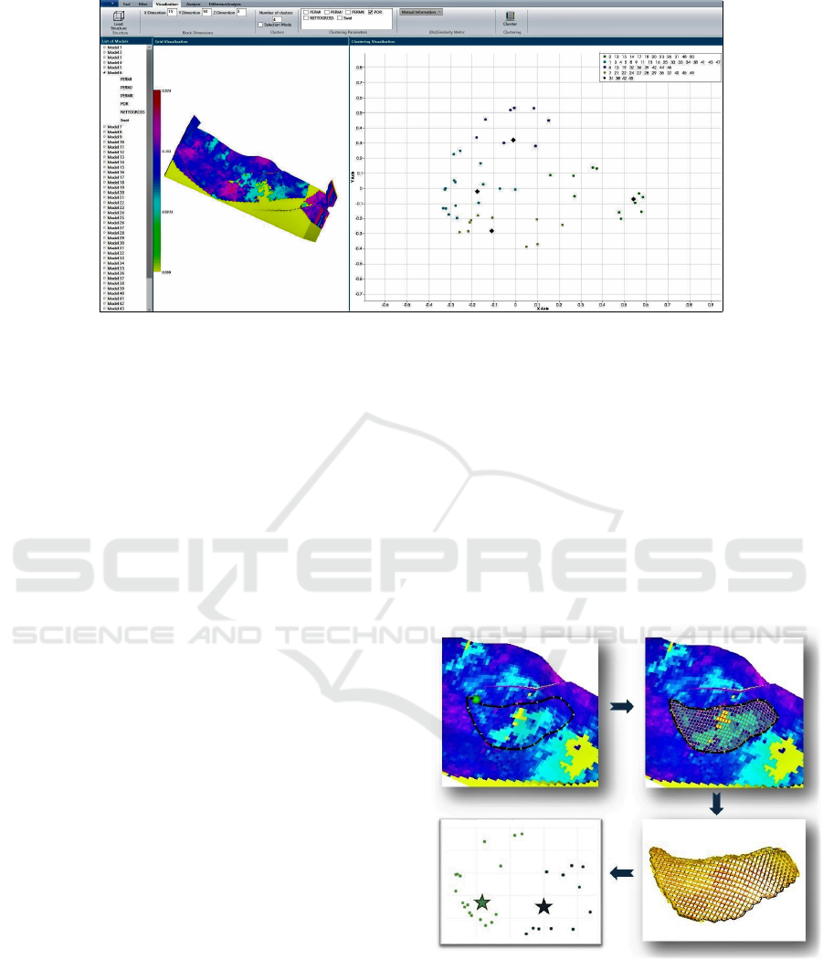
Figure 14: Projection and clustering of loaded models.
can import any number of the models into the applica-
tion. Each model can be visualized in 3D. The color
scale shows the value of a selected property. Warm
colors show the higher value of the selected property
and in reverse for the cool colors. There are two main
visual analytical processes in this prototype: selection
process and comparison analysis.
8.1 Selection Process
The selection process consists of two main steps:
calculation of (dis)similarity and clustering. Two
main parameters are specified by the users: block
size and reservoir property(ies). The default optimal
block size is calculated in the background (using the
entropy-based approach mention in section 5.2) and
is provided in the interface as a suggestion. However,
users can also change that according to their knowl-
edge of the reservoir. Block size is specified by three
values for each 3D dimension: x, y, and z. Each of
them can be changed by the users interactively. The
other parameter that should be specified is the static
reservoir property(ies) that are used for the distance
calculation. Users can specify one or more number of
properties (R3).
After that, the number of clusters should be spec-
ified by the user, that is determined based on user’s
budget and time for running flow simulation. The
clustering outcome is presented on a diagram in the
2D view. Each point in the diagram corresponds to a
projected geological model. The color legend on the
2D diagram shows the clustering results (Figure 14).
In result, the median member of each cluster is se-
lected as the representative member of that cluster
(R1). Since the calculated distances are mapped to
the 2D view, it also helps the users to have an overall
representation of models.
According to our discussions with domain ex-
perts, they need to perform selection process based
on a specific region of a model. This is because
they are sometimes dealing with very large reservoirs,
and not the whole reservoir geometry is important to
them. For instance, in a substantially large reservoir
model, the engineers are usually interested in the ar-
eas around wells. To leverage this requirement, the
users can freely sketch an arbitrary 3D area on the
model. And then the selection process constrains the
calculation of (dis)similarity only to that specific re-
gion (R4). (Figure 15)
Figure 15: Filtering process for an arbitrary area of interest.
8.2 Comparison Analysis
In addition to the calculated distance values, the users
also frequently need to get more detailed spatial in-
formation about the differences between models. For
instance, the engineers might need to get some in-
IVAPP 2018 - International Conference on Information Visualization Theory and Applications
82

sights into the regions that the models show a signif-
icant difference. To provide this feature, users can
select any number of models from the 2D view. A
3D similarity map is calculated and visualized for the
specific selected models (R5). In the similarity map,
the users can observe the local similarity between the
models - i.e., which parts of the model contribute
additional weights in the similarity and dissimilarity
calculations. For instance, Figure 16 is a similarity
map for four selected models. The color scale shows
the amount of mutual information between all these
four models. The results show that these models are
very similar in the red and dark blue areas, and they
are very different light green areas. This feature not
only helps identify the important regions of models
but also utilizes a useful feature of mutual informa-
tion that can be calculated between multiple objects
at the same time with multivariate mutual information
techniques (Batina et al., 2011).
Figure 16: Similarity map for the selected models.
9 CONCLUSION AND FUTURE
WORKS
In this paper, we introduced a new visual analytical
framework for selecting a few representative models
from an ensemble of geostatistical models that repre-
sents the overall production uncertainty. To achieve
this purpose, a new block wise (dis)similarity metric
was defined based on mutual information. This met-
ric is projected to a lower dimension using the MDS
technique, and then the new projected distance is used
in a kernel KMC algorithm to group models based on
their distances. The proposed workflow was evalu-
ated using some datasets generated from various geo-
statistical algorithms. The results of the case stud-
ies show that our technique is accurate and efficient
in comparison to the existent techniques. In the fu-
ture, with the help of domain experts, we need to find
more adequate parameters for uncertainty assessment
of geological models. Moreover, regarding the appli-
cation, we need to support comparing of clustering
results, and in continuing that, provide more infor-
mation to the users such as what is the best number
of clusters, or what are the effective parameters. We
will also further evaluate our application using a for-
mal user study, that helps identify additional weak-
ness and strengths of the current application and pro-
cess.
ACKNOWLEDGMENT
We wish to thank the anonymous reviewers for their
constructive comments, CMG (Computer Modelling
Group Ltd.) for providing the reservoir data sets and
Masoud Zehtabioskuie for his valuable help and feed-
back on the implementation of the application. This
research was supported in part by NSERC.
REFERENCES
Ballin, P., Journel, A., Aziz, K., et al. (1992). Prediction of
uncertainty in reservoir performance forecast. Journal
of Canadian Petroleum Technology, 31(04).
Batina, L., Gierlichs, B., Prouff, E., Rivain, M., Standaert,
F.-X., and Veyrat-Charvillon, N. (2011). Mutual in-
formation analysis: a comprehensive study. Journal
of Cryptology, 24(2):269–291.
Bordoloi, U. D., Kao, D. L., and Shen, H.-W. (2004). Vi-
sualization techniques for spatial probability density
function data. Data Science Journal, 3:153–162.
Bruckner, S. and M
¨
oller, T. (2010). Isosurface similar-
ity maps. In Computer Graphics Forum, volume 29,
pages 773–782. Wiley Online Library.
Bruckner, S. and Moller, T. (2010). Result-driven explo-
ration of simulation parameter spaces for visual ef-
fects design. IEEE Transactions on Visualization and
Computer Graphics, 16(6):1468–1476.
Caers, J. (2011). Modeling Uncertainty in the Earth Sci-
ences. Wiley Online Library.
Cole-Rhodes, A. A., Johnson, K. L., LeMoigne, J., and Za-
vorin, I. (2003). Multiresolution registration of remote
sensing imagery by optimization of mutual informa-
tion using a stochastic gradient. IEEE transactions on
image processing, 12(12):1495–1511.
Correa, C. D., Chan, Y.-H., and Ma, K.-L. (2009). A frame-
work for uncertainty-aware visual analytics. In IEEE
VAST, pages 51–58.
Cover, T. M. and Thomas, J. A. (2012). Elements of infor-
mation theory. John Wiley & Sons.
Demir, I., Dick, C., and Westermann, R. (2014). Multi-
charts for comparative 3d ensemble visualization.
IEEE Transactions on Visualization and Computer
Graphics, 20(12):2694–2703.
Dhillon, I. S., Guan, Y., and Kulis, B. (2004). Kernel k-
means: spectral clustering and normalized cuts. In
Proceedings of the tenth ACM SIGKDD international
conference on Knowledge discovery and data mining,
pages 551–556. ACM.
A Visual Analytics Framework for Exploring Uncertainties in Reservoir Models
83

Fenwick, D. and Batycky, R. (2011). Using metric space
methods to analyse reservoir uncertainty. In Proceed-
ings of the 2011 Gussow Conference.
Fofonov, A., Molchanov, V., and Linsen, L. (2016). Visual
analysis of multi-run spatio-temporal simulations us-
ing isocontour similarity for projected views. IEEE
transactions on visualization and computer graphics,
22(8):2037–2050.
France, S. L. and Carroll, J. D. (2011). Two-way multidi-
mensional scaling: A review. IEEE Transactions on
Systems, Man, and Cybernetics, Part C (Applications
and Reviews), 41(5):644–661.
Goshtasby, A. A. (2012). Image registration: Principles,
tools and methods. Springer Science & Business Me-
dia.
Haidacher, M., Bruckner, S., Kanitsar, A., and Gr
¨
oller,
M. E. (2008). Information-based transfer functions for
multimodal visualization. In VCBM, pages 101–108.
Honarkhah, M. and Caers, J. (2010). Stochastic simula-
tion of patterns using distance-based pattern model-
ing. Mathematical Geosciences, 42(5):487–517.
Huttenlocher, D. P., Klanderman, G. A., and Rucklidge,
W. J. (1993). Comparing images using the hausdorff
distance. IEEE Transactions on pattern analysis and
machine intelligence, 15(9):850–863.
Idrobo, E. A., Choudhary, M. K., Datta-Gupta, A., et al.
(2000). Swept volume calculations and ranking of
geostatistical reservoir models using streamline sim-
ulation. In SPE/AAPG Western Regional Meeting. So-
ciety of Petroleum Engineers.
Kao, D., Luo, A., Dungan, J. L., and Pang, A. (2002). Vi-
sualizing spatially varying distribution data. In Infor-
mation Visualisation, 2002. Proceedings. Sixth Inter-
national Conference on, pages 219–225. IEEE.
Kehrer, J., Filzmoser, P., and Hauser, H. (2010). Brush-
ing moments in interactive visual analysis. In Com-
puter Graphics Forum, pages 813–822. Wiley Online
Library.
Kehrer, J. and Hauser, H. (2013). Visualization and vi-
sual analysis of multifaceted scientific data: A sur-
vey. IEEE transactions on visualization and computer
graphics, 19(3):495–513.
Kehrer, J., Muigg, P., Doleisch, H., and Hauser, H. (2011).
Interactive visual analysis of heterogeneous scientific
data across an interface. IEEE Transactions on Visu-
alization and Computer Graphics, 17(7):934–946.
Li, S., Deutsch, C. V., and Si, J. (2012). Ranking geostatisti-
cal reservoir models with modified connected hydro-
carbon volume. In Ninth International Geostatistics
Congress, pages 11–15.
Lin, D. (1998). An information-theoretic definition of sim-
ilarity. In ICML, volume 98, pages 296–304. Citeseer.
Love, A. L., Pang, A., and Kao, D. L. (2005). Visualizing
spatial multivalue data. IEEE Computer Graphics and
Applications, 25(3):69–79.
MacKay, D. J. (2003). Information theory, inference and
learning algorithms. Cambridge university press.
Nocke, T., Flechsig, M., and Bohm, U. (2007). Visual ex-
ploration and evaluation of climate-related simulation
data. In 2007 Winter Simulation Conference, pages
703–711. IEEE.
Rahim, S. and Li, Z. (2015). Reservoir geological uncer-
tainty reduction: an optimization-based method using
multiple static measures. Mathematical Geosciences,
47(4):373–396.
Scheidt, C. and Caers, J. (2010). Bootstrap confidence in-
tervals for reservoir model selection techniques. Com-
putational Geosciences, 14(2):369–382.
Scheidt, C., Caers, J., et al. (2009). Uncertainty quantifica-
tion in reservoir performance using distances and ker-
nel methods. SPE Journal, 14(04):680–692.
Sch
¨
olkopf, B., Smola, A., and M
¨
uller, K.-R. (1998). Non-
linear component analysis as a kernel eigenvalue prob-
lem. Neural computation, 10(5):1299–1319.
Scholkopf, B. and Smola, A. J. (2001). Learning with ker-
nels: support vector machines, regularization, opti-
mization, and beyond. MIT press.
Shawe-Taylor, J. and Cristianini, N. (2004). Kernel methods
for pattern analysis. Cambridge university press.
Wang, C., Yu, H., and Ma, K.-L. (2008). Importance-driven
time-varying data visualization. IEEE Transactions on
Visualization and Computer Graphics, 14(6):1547–
1554.
Williams, C. K. (2002). On a connection between kernel pca
and metric multidimensional scaling. Machine Learn-
ing, 46(1-3):11–19.
Wilson, A. T. and Potter, K. C. (2009). Toward visual anal-
ysis of ensemble data sets. In Proceedings of the 2009
Workshop on Ultrascale Visualization, pages 48–53.
ACM.
Yazdi, M. M. and Jensen, J. L. (2014). Fast screening of
geostatistical realizations for sagd reservoir simula-
tion. Journal of Petroleum Science and Engineering,
124:264–274.
Zhang, J., Huang, H., and Wang, J. (2010). Manifold learn-
ing for visualization and analyzing high dimensional
data. IEEE.
IVAPP 2018 - International Conference on Information Visualization Theory and Applications
84
