
Dynamic Pricing Strategy for Electromobility using Markov Decision
Processes
Jan Mrkos, Anton
´
ın Komenda and Michal Jakob
Artificial Intelligence Center, Faculty of Electrical Engineering, Czech Technical University in Prague, Czech Republic
Keywords:
Electric Vehicles, Demand-response, Dynamic Pricing, Charging, MDP, Markov Decision Process.
Abstract:
Efficient allocation of charging capacity to electric vehicle (EV) users is a key prerequisite for large-scale
adaption of electric vehicles. Dynamic pricing represents a flexible framework for balancing the supply and
demand for limited resources. In this paper, we show how dynamic pricing can be employed for allocation of
EV charging capacity. Our approach uses Markov Decision Process (MDP) to implement demand-response
pricing which can take into account both revenue maximization at the side of the charging station provider
and the minimization of cost of charging on the side of the EV driver. We experimentally evaluate our method
on a real-world data set. We compare our dynamic pricing method with the flat rate time-of-use pricing that
is used today by most paid charging stations and show significant benefits of dynamically allocating charging
station capacity through dynamic pricing.
1 INTRODUCTION
Electrification of personal transportation is commenc-
ing. There is a multitude of reasons, primarily en-
vironmental concerns, energy supply independence,
and overall falling costs of production of both elec-
tric vehicles and the needed energy. Hand in hand
with the clear benefits of a wide-spread deployment of
electric vehicles (EVs) come many challenges. One
of the most pressing problems is how to efficiently
and cheaply distribute the energy from often unstable
renewable sources to the EVs.
To illustrate the gravity of the situation, let us take
the recent target to charge future EVs by no less than
300kW (Dyer et al., 2013). Provided a charging sta-
tion with ten charging slots, we get to 3MW power
intake if all the slots are charging EVs in parallel. For
a comparison, an average instantaneous power con-
sumption
1
of a U.S. household is about 1.2kW. The
costs of upgrading the distribution network to cover
such intakes would be extreme, on par with build-
ing the grid for additional three times the number of
households
2
.
1
Based on the 2015 statistics of the U.S. Energy In-
formation Administration: https://www.eia.gov/tools/faqs/
faq.php?id=97&t=3https://www.eia.gov/tools/faqs/faq.php
?id=97&t=3
2
Based on the IEEE Spectrum article: http://
spectrum.ieee.org/transportation/advanced-cars/speed-
Provided that the charging stations are not perma-
nently fully occupied by EVs, an alternative to up-
grading the grid is to charge stationary batteries at
charging station, which are later used to fast charge
EVs. In this approach, the initial costs of the up-
grade of the grid are transferred to charging station
owners in the cost of stationary batteries. Another
approach is to use grid-centric methods ensuring fair-
ness of charging such as the packetized charging man-
agement (Rezaei et al., 2014). However, such meth-
ods do not guarantee the charging service capacity,
therefore the charging duration can not be guaranteed.
Existing regulations and laws design the overall
mechanism for the allocation of charging resources.
Within the rules of this mechanism, participants in
this mechanism are free to act in a way that pro-
motes their self-interests. These participants are
power distribution service operators, charging service
providers, and EV drivers responsible for charging
their cars. However, self-interested strategies em-
ployed by the participants can be dangerous to the
system as a whole. Multi-agent paradigm is suitable
to efficiently balance the supply of the (renewable)
power and EV charging demand. More precisely, the
field of multi-agent resource allocation (Chevaleyre
et al., 2006) provides techniques for solving problems
bumps-ahead-for-electricvehicle-charging
http://spectrum.ieee.org/transportation/advanced-cars/
speed-bumps-ahead-for-electricvehicle-charging
Mrkos, J., Komenda, A. and Jakob, M.
Dynamic Pricing Strategy for Electromobility using Markov Decision Processes.
DOI: 10.5220/0006601505070514
In Proceedings of the 10th International Conference on Agents and Artificial Intelligence (ICAART 2018) - Volume 2, pages 507-514
ISBN: 978-989-758-275-2
Copyright © 2018 by SCITEPRESS – Science and Technology Publications, Lda. All rights reserved
507

with self-interested agents.
We base our approach to dynamic pricing on the
pricing of charging services as whole. This means
that we do not consider the charging station to be sell-
ing electricity with price per kWh as is currently the
norm. Instead, in our view, the charging station is sell-
ing a charging service that has multiple parameters
that include time of day, volume of consumed elec-
tricity etc. This approach does not directly depend
on the details of the low-level battery charging pat-
terns and its optimization as proposed in (Cao et al.,
2012). (Li et al., 2014) suggests an idea similar to
our approach in the locational pricing; however, their
method is based on the solution of nonlinear opti-
mization towards the social welfare to get charging
prices. Our approach solves the same problem as a
solution to a set of decentralized Markov Decision
Processes (MDPs), where the resulting decisions are
prices of charging services at various times.
In this paper, we provide an experimental com-
parison of the MDP demand-response pricing strategy
applicable in the context of multi-agent resource allo-
cation for electromobility and today widespread flat
rate time-of-use pricing (Versi and Allington, 2016).
2 DEMAND-RESPONSE PRICING
Economics, revenue management, and supply chain
management have extensively studied demand-
response pricing mechanisms of various kinds of ser-
vices (Albadi and El-Saadany, 2008; McGill and
van Ryzin, 1999). These fields recognize demand-
response pricing as a critical lever for influencing
the behavior of buyers. For this quality, we choose
demand-response pricing as a way of dealing with in-
creasing loads on the power grid caused by uptake of
EVs.
To put the charging services pricing into context,
we can view it as pricing of perishable goods, such as
seasonal clothing, hotel rooms or airline tickets (Sub-
ramanian et al., 1999). These goods have value only
until a certain point in time. For clothing, that is the
end of the season, for airline tickets, it is the depar-
ture of the airplane. In the case of charging stations,
the commodity is the charging resources available in
a given time window. With perishable products, the
goal is to sell the available stock for a profit before
the stock expires. Same with the charging services,
charging resources are a missed profit opportunity if
they are left unused at the end of some time window.
Pricing of airline tickets has been extensively
studied in different variations and with focus on vari-
ous aspects of the problem (Chiang et al., 2007). The
Figure 1: Difference between airline pricing and charging
station pricing. Green rectangles show valid bookings. Seat
bookings do not significantly affect bookings of other seats
(except for large group bookings). On the other hand, a
booking of short charging sessions and 1:00 and 4:00 blocks
bookings of longer charging sessions shown in red.
first step is usually the construction of an approximate
model of user behavior (such as customer price sen-
sitivity, seasonality of demand, no shows, etc.). Next,
airlines need to determine how many tickets at which
price to sell through the maximization of expected
revenue. In brief, optimal rule for accepting or re-
jecting bookings is as follows: “Is the profit from this
booking greater or smaller than the expected profit
from this seat that we could get later? Confirm the
booking now if the profit is bigger than the expected
profit later. If it is smaller, deny this booking.”
However, each accepted or rejected booking can
influence following bookings as consecutive cus-
tomers are not able to book seats at the same price.
If we include connecting flights and group bookings
into the problem, pricing decisions can have a domino
effect on the pricing in the whole network of an air-
line operator. Although the problem can look simple,
due to this knock-down effect, the survey (McGill and
van Ryzin, 1999) notes the complexity of this issue.
For this reason, most work on this subject restricts the
problem in some way.
In the following sections, we approach the charg-
ing station pricing strategy in a similar way to how
airline revenue management approaches the pricing
of airline tickets. Both problems focus on perish-
able goods where the knockdown effect plays a role
as both bookings of airline tickets and bookings of
charging station can affect following sales.
Similarly to airline revenue management, we do
not directly consider competition between different
service providers. We aggregate charging station cus-
tomers (whose actions are based the options offered
by different service providers as well as individual
circumstances) in an environment model that adjusts
demand as a response to changing price.
An important distinction between the airline pric-
ing and charging station pricing is the interconnected-
ICAART 2018 - 10th International Conference on Agents and Artificial Intelligence
508

ness of the bookings in the case of charging services;
this is not present with the sales of the airline tick-
ets. In the case of the airline tickets, it is not particu-
larly important which seat (in a given class) was sold
as booking of single seat does not block booking of
surrounding seats. This distinction is illustrated in
Figure 1.
3 PRICING STRATEGY
In the next section, we focus on the formalization and
modeling of the pricing strategies as Markov Decision
Processes (MDP)(Bellman, 1957).
3.1 Demand-response Pricing Strategy
We focus on the demand-response pricing strat-
egy (Albadi and El-Saadany, 2008) for single charg-
ing station. As input, we use a discretization of possi-
ble charging parameters (time, duration and location
of charging), current and historical utilization of sin-
gle charging station and the expected price elasticity
of the demand for charging services.
The goal of the pricing strategy described below is
the maximization of charging station revenue within
particular time horizon. However, other optimization
criteria are possible to achieve different goals. For
example, a publicly owned charging station that is
not concerned with profits may attempt to maximize
charging station utilization or minimize waiting times
at the charging station.
3.2 Problem Formalization
In this section, we formalize the problem of dynamic
pricing of charging station offers. In this formaliza-
tion, our focus is on the offers that use the uniform
discretization of time and some form of discretiza-
tion of the other offer parameters. Regular structur-
ing in time simplifies the formalization. We consider
the set T of times t
1
,t
2
, . . . ,t
n
for which the prices
p
1
, p
2
, . . . , p
n
need to be determined.
The times in T denote the starting times of time
intervals of the same length that start at time t
i
and
end at time t
i+1
. For simplicity, we denote both the
time interval and the associated start time with t
i
. c
i
is the expected free charging capacity of the charging
station in each time interval t
i
.
In this formalization, we use the symbol c
i
, the ex-
pected free capacity to be the aggregate of all charging
station constraints, such as power grid capacity or the
number of available charging connectors.
Customers may book charging in any future time
interval. Thus, we will denote price and capacity as
functions p(t
i
, τ) and c(t
i
, τ), meaning the price or ca-
pacity of ith time interval at time τ ∈ T . Fixing the
time τ, both price and capacity functions are elements
of the space of step functions over real numbers L .
Given an offer, each reservation r
j
= (r
0
j
, r
1
j
, τ
j
) ∈
R is made for one or more consecutive time intervals,
starting at time interval r
0
j
and ending in r
1
j
. The ar-
rival of a reservation is denoted τ
j
. The price of the
reservation π(r
j
) is the sum of prices associated with
the time intervals at the time of the reservation:
π(r
j
= (r
0
j
, r
1
j
, τ
j
)) =
r
1
j
∑
t=r
0
j
p(t, τ
j
)
Reservations arrive randomly according to a de-
mand distribution that is dependent on the price func-
tion as well as external factors. The set of reservations
R depends on the pricing function because changes
to the price influence demand. Thus, R is a function
R(p) : L × T → 2T × T × T , where 2T × T × T is the
superset of the set of all possible reservations. The
initial free capacity of the time interval relies on the
state of the grid. We model this as stationary distribu-
tion.
The goal of the charging station is to maximize
profits. In each time interval, charging station needs
to cover the ground cost of maintaining the infras-
tructure denoted Γ
g
. During charging, a charging sta-
tion needs to pay for the electricity consumed from
the grid γ(r
j
). This cost is unique to each charging
session as it depends on the total charge delivered to
the EV and possibly variable price of electricity and
charging rate. Given that the price π(r
j
) of a reser-
vation r
j
, profit or loss at the end of the time horizon,
after n time intervals, can be written as the sum across
all reservations:
Π = −nΓ
g
+
∑
r
j
∈R
π(r
j
) − γ(r
j
)
However, this point of view of the profit is not par-
ticularly useful for optimization. As each price π(r
j
)
is calculated as the sum of prices of booked time inter-
vals, we can rewrite the profit as a function of pricing
of time intervals:
Π(p) = −nΓ
g
+
∑
r
j
∈R(p)
r
1
j
∑
t=r
0
j
p(t, τ
j
) − γ(r
j
)
The optimization goal of the pricing is then:
p
0
= argmax
p∈L
Π(p)
Dynamic Pricing Strategy for Electromobility using Markov Decision Processes
509

Finding optimal pricing function is not an easy
task. The pricing function is part of the innermost
sum in the calculation of Π. The sum itself is also de-
pendent on p, as the set of reservations R is dependent
on p. In fact, the set of reservations is dependent on p
through the actions and responses of individual cus-
tomers. However, it would be challenging to model
behavior of each customer to get optimal pricing strat-
egy.
To make the problem tractable, we aggregate be-
havior of a multitude of customers into the probability
distributions that describe the behavior of customers
together. As such, we can no longer maximize the
profit in absolute numbers. Instead, we maximize the
expected profit (in the statistical sense):
p
0
= argmax
p∈L
E(Π(p)) (1)
The framework that deals with problems posed
this way is the framework of Markov Decision Pro-
cesses.
3.3 Modeling as a Markov Decision
Process
The described optimization problem is a complex one.
To solve it, we choose to model the charging ser-
vices pricing problem as a Markov Decision Process
(MDP) (Bellman, 1957; Puterman., 1994). First, we
decompose the optimization problem into a sequence
of decisions, where at each time point τ, we need to
select new pricing function p ∈ L . Markov Decision
Processes provide a framework for modeling a broad
range of sequential decision problems, where an agent
must submit a sequence of decisions as responses to
the developing environment.
An MDP is a tuple
h
S, A, R, P, s
0
i
, where S is a fi-
nite set of states, A is a finite set of actions; P : S×A ×
S → [0, 1] is the transition function forming the transi-
tion model giving a probability P(s
0
|s, a) of getting to
the state s
0
from the state s after application of the ac-
tion a; and a reward function R : S ×A × S → R. Start-
ing in initial state s
0
, any action from A can be chosen.
Based on this action, the system develops and moves
to the next state where another action can be applied.
During the move, the reward can be received based on
the R(s, a, s
0
) function.
When solving the MDP, the goal is to select a se-
quence of actions that will in expectation lead to the
highest accumulated reward.
For the implementation, we consider a charging
station with integer capacity between 0 and c
max
and
possible prices being integers between 1 and p
max
.
We consider a single day of 24 time intervals, each
1 hour long. For computational feasibility reasons,
we split the MDP into multiple MDPs, one for each
time window. This splitting gives us 24 MDPs, each
responsible for setting the price of the corresponding
time window. Each MDP generates a decision pol-
icy for its own time window. While these policies are
optimal in a sense that they maximize the reward in
given time window, together they may not maximize
the revenue in the whole day.
MDP-1 is in charge of setting the price between
00:00 and 01:00, MDP-2 for setting the price in the
time window between 01:00 and 02:00 and so on. As
the bookings arrive ahead of the charging, we include
time t to the kth time window in the state of the kth
MDP. For example, in our experiments, at the time
between 13:00 and 14:00, time t to MDP-18 is 4.
State s of MDP-k is thus defined by the capacity,
price and time; s = (c, p,t). The actions are changes
to the price in the kth time interval, that is, a = p
0
. The
transition model for the kth MDP, P
k
(s
0
|s, a) then de-
termines, given the current price, capacity and time to
the kth time interval, whether somebody books charg-
ing (which reduces capacity in the time window.). We
calculate the transition probabilities from the given
price elasticity function P
e
(p) and discrete historical
probability D
k
(t) of a booking arriving t ahead of kth
time window:
P
k
((c − 1, p
0
,t − 1)|(c, p, t), p
0
) =P
e
(p)D
k
(t),
c > 0, t > 1
P
k
((c, p
0
,t − 1)|(c, p, t), p
0
) =1 − P
e
(p)D
k
(t),
t > 0
P
k
((c
0
, p
0
,t
0
)|(c, p,t), p
0
) =0 otherwise
D
k
(t) give the probability of a booking for charg-
ing during kth time interval arriving t ahead of the kth
time interval.Values of D
k
(t) are taken from the his-
torical data. The use of D
k
(t) in the transition func-
tion forms a simplified demand model that models
the distribution of demand within one day, but one
that is independent of the absolute demand expected
within this day. Price elasticity function P
e
(p) gives
the probability that given price p a customer will ac-
cept the price of the booking.
Instead of maximizing the profit of the whole day
(in the sense of Equation 1), each MDP factor max-
imizes the profit in given time window. This adjust-
ment is an important omission regarding optimality
of the resulting pricing. As Figure 1 shows, sales of
time windows affect the value of the neighboring time
windows. However, as we will show in Section 4,
even in this factored form with simple demand model,
MDP demand-response pricing can bring some bene-
fits. In the model, splitting of the MDP into MDP
ICAART 2018 - 10th International Conference on Agents and Artificial Intelligence
510

Table 1: Summary statistics of the E-WALD data for the
selected charging station with three charging points.
CS Dataset Statistics Mean Std
Charging session duration 0.726 h 0.794 h
Charge per charging session 6.72 kWh 5.19 kWh
# of daily charging sessions 2.53 1.49
Figure 2: Histogram of the charging session start times in
the E-WALD dataset for the selected charging station.
factors means that changes to capacity and price do
not affect on the neighboring prices.
We find the optimal policies for MDP-1 to MDP-
24 through policy iteration. We implemented all
structures and algorithms in Python, using commonly
used Python packages such as NumPy (van der Walt
et al., 2011) and Pandas (McKinney, 2011). Policy
iteration algorithm that we used is from the pymdp-
toolbox
3
.
4 EXPERIMENTS
We evaluate the MDP dynamic pricing algorithm on
real data provided by E-WALD
4
, EV charging station
provider in Germany. First, we provide summarizing
statistics of the dataset and describe the preprocessing
we performed on the data. Then we describe the ex-
periments we conducted with the data and the results
we obtained.
4.1 Dataset
The dataset contains information on charging sessions
realized at one of the E-WALD charging stations.
This information includes timestamps of the begin-
ning and the end of each charging session, the sta-
tus of the electricity meter at the beginning and the
end of the charging session and anonymized identifier
of a user who activated the charging session. In the
3
https://github.com/sawcordwell/pymdptoolbox
4
We would like to thank E-WALD for providing us with
the charging data for this study.
preprocessing step, we remove clearly erroneous data
points, (such as charging sessions with negative du-
ration) and merge some short charging sessions with
following charging sessions if the same customer ini-
tiated both sessions.
The summary statistics of the dataset can be found
in Table 1. Histogram of charging session start times
can be seen in Figure 2.
The particular charging station dataset does not
contain any pricing information about the charging
sessions. However, E-WALD uses only flat rate pric-
ing in all their pricing stations.
4.2 Experimental Setup
In our experiments, we compare the performance of
the flat rate pricing to the MDP based dynamic pric-
ing. To compare their performance we use four met-
rics, charging station revenue, charging station uti-
lization time, charge delivered by the charging station
and price per unit of energy sold by the charging sta-
tion. A detailed description of these metrics is given
in Table 2.
We use the real E-WALD charging station data to
simulate 24 hour period of the charging station oper-
ation. As the data was collected at charging station
with three charging slots, in our experiments we con-
sider our station to have three charging points. That
is, we use c
max
= 3 and p
max
= 5. We consider the
charging points to be capable of realizing any charg-
ing session recorded in our dataset. This means that
at most three charging sessions can be realized at
any point in time. In our simulation, customers book
charging sessions ahead of time. Charging station re-
jects the booking if all three charging points are al-
ready booked for any portion of the requested time.
If the station can realize the booking, pricing scheme
is used to determine the price of the charging session
which the station offers to the customer. Based on
this price, the customer either accepts or rejects the
offer. Price elasticity of demand described below de-
termines whether the offer is accepted or rejected by
the customer.
To make it possible for users to plan their trips in
the environment where the charging capacity may not
be readily available, we use ahead of time bookings
in our simulation. We simulate how much ahead each
customer books the charging session by drawing from
the uniform distribution. The maximum period ahead
of which customer can book a charging session is in
our experiments set to 6 hours. The time of the book-
ings determines the order of the arrival of the book-
ings to the.
The simulation starts by drawing n charging ses-
Dynamic Pricing Strategy for Electromobility using Markov Decision Processes
511
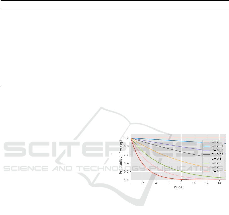
Table 2: Description of evaluation metrics.
Metric Description
CS Revenue Revenue of the charging station is the sum of prices of all charging sessions. We do not
express price in any currency. Instead, we use unit price as a basic unit. Revenue is
directly dependent on the selected pricing scheme.
CS Utilization Measured in hours, it is the added duration of all charging sessions realized by the
charging station. This as a proxy of a social welfare of the EV drivers achieved through
various pricing schemes. The higher the utilization, the more of the EV driver charging
demand was satisfied by the charging station.
Delivered Charge Measured in kWh, it is the charge delivered to all of the charging station customers.
Delivered charge is another proxy of a social welfare of the EV drivers realized by various
pricing schemes. The higher the delivered charge, the more of the EV charging demand
was satisfied by the charging station. Because of each EV charging with different
charging rate, this information complements the CS Utilization metric.
Energy price Average price per unit of energy across all charging sessions realized by the CS.
sions from the dataset. As can be seen from Table 1,
the mean number of customers at the charging station
is quite small. Also, the dataset does not give us any
information about the unsatisfied demand for charg-
ing services. Thus, in most of our experiments, we
use higher values of n so that all demand cannot be
satisfied by the given charging station.
Normalized histogram in Figure 2 and the sim-
ulated booking times are the basis of the histori-
cal probability D
k
(t) of a booking request arriving t
ahead of kth time window.
The MDP dynamic pricing uses different price for
every hour. To get the price of the charging session,
we first split the charging session into segments that
correspond to the various dynamic prices. The cor-
responding hourly rate then multiplies the length of
each segment. Adding the partial prices together gets
us the price of the charging session offered to the user.
For the flat rate pricing, the duration of the charging
session in hours is multiplied by the hourly rate.
When the customer receives the offered price, he
can accept or reject the offer. We simulate this using
the price elasticity of demand curve. The price elas-
ticity function we use is P
e
(x) = e
−Cx
.
Because we do not know the real price elasticity
of demand for EV charging services and we can not
estimate it from data, we experiment with multiple
values of C. The different values of C and the corre-
sponding shapes of price-elasticity curves are shown
in Figure 3. Having the price of the charging session,
we apply the price elasticity function to this price.
The resulting number is a probability that the cus-
tomer accepts the offer. If the user accepts the of-
fer, the charging session is added to the other already
booked charging sessions. Rejected offer is discarded
and no longer used by the system. For C = 0, we talk
about inelastic demand as the customer will accept
any price. At C = 0.5 the demand is highly elastic as
small changes to the price have a big effect on users
acceptance or refusal of the offer. For comparison,
the price elasticity of demand for gas station services
is usually described as relatively inelastic, meaning
low values of C (Lin Lawell and Prince, 2013).
Figure 3: Price elasticity of demand curves for different val-
ues of the C parameter.
4.3 Results
To compare the performance of the MDP dynamic
pricing and the flat rate pricing, we experimented with
various numbers of customers and various parameters
of price elasticity of these customers. In each experi-
ment, we compare the MDP dynamic pricing that can
set price in each time window to an integer value be-
tween 1 and 5. We compare it to the flat rate pricing
that uses flat rates between 1 and 5.
For the first experiment, we fixed the price elas-
ticity parameter to C = 0.1 and varied the number of
customers arriving per day from 2 to 80. For the sec-
ond experiment, we varied the number price elasticity
parameter C through values given in Figure 3. We
fixed the number of booking to 40.
Each data point in Figures 4 and 5 is an average of
ICAART 2018 - 10th International Conference on Agents and Artificial Intelligence
512
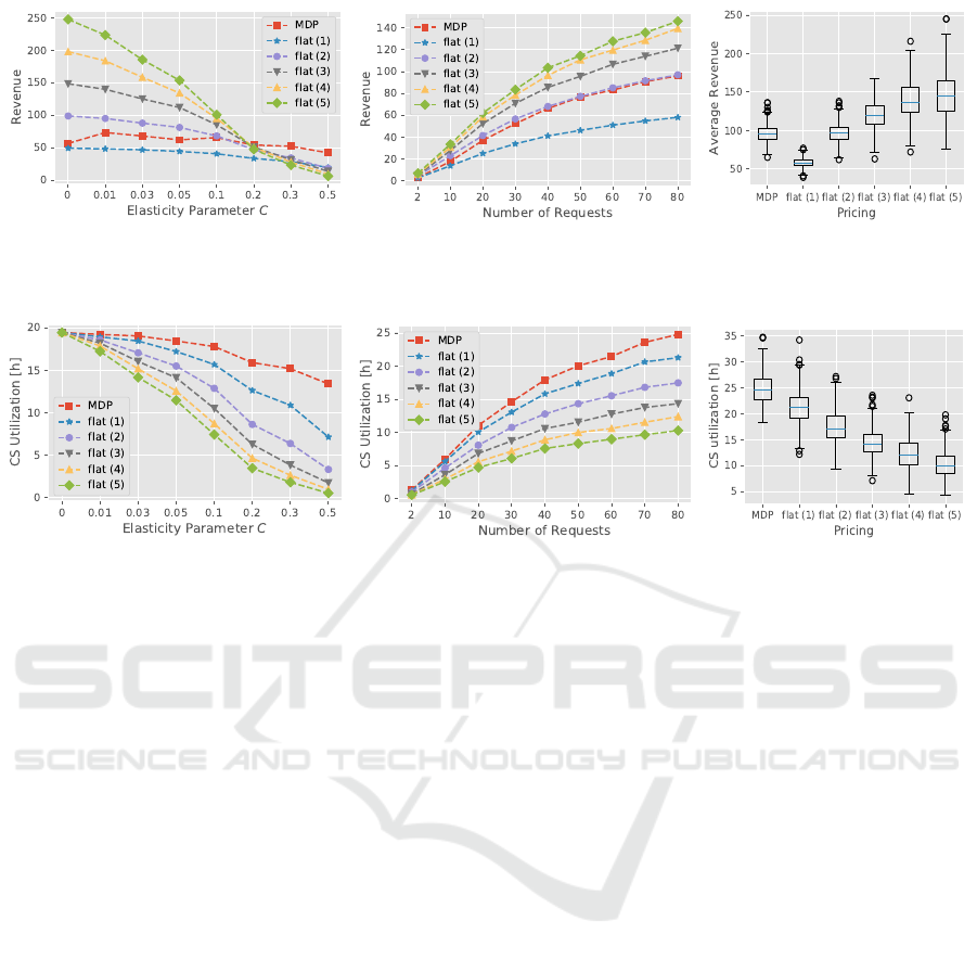
Figure 4: Performance in terms of revenue of the MDP dynamic pricing compared to the performance of the flat rate during
one simulated day. The graphs are based on 400 runs with a random selection of booking requests from the E-WALD dataset.
Price elasticity parameter C = 0.1and n = 40 booking requests in plots where these parameters are not on axis.
Figure 5: Performance in terms of CS utilization of the MDP dynamic pricing compared to the performance of the flat rate
during one simulated day. The graphs are based on 400 runs with a random selection of booking requests from the E-WALD
dataset. Price elasticity parameter C = 0.1and n = 40 booking requests in plots where these parameters are not on axis.
400 runs. In each run, we picked the booking requests
randomly from the full E-WALD dataset. For price
elasticity parameter C = 0.1 and 40 requests we give
the quartiles of the evaluation metrics.
As could be expected, increasing the number of
booking requests increases revenue, utilization and
delivered charge for all pricing schemes. Figure 4 for
revenue and Figure 5 for CS utilization illustrate this,
curves for delivered charge display the same trends as
figures for utilization.
Note that while the revenue is lower for the MDP
demand-response pricing for the lower price elasticity
curves (C < 0.2), the charging station utilization and
delivered charge are better across all values of C. The
utilization and delivered charge are same for all pric-
ing schemes when C = 0; that is, when the demand
is inelastic, customers always accept the offered price
and the charging capacity is distributed solely on the
first come, first serve basis.
For the experiment with variable elasticity param-
eter C, the downslope trend of the utilization and
delivered charge with increasing elasticity are to be
expected, given the fixed number of 40 booking re-
quests at average duration 0.726 (the maximal theo-
retical utilization with three charging points would be
3 ∗ 24). As the price elasticity increases, the likeli-
hood of any given customer booking for given price
becomes lower.
Another notable result is that while the MDP price
per kWh is for most values of C comparable to the flat
rate of price 1, the revenue of MDP is consistently
higher than the revenue of the flat rate of 1.
The results show that that in simulation, the MDP
dynamic pricing will return greater revenue than flat
rates with a price higher than one only if the demand
for EV charging is somewhat elastic (elasticity pa-
rameter C ≥ 0.2, Figure 3). However, dynamic pric-
ing improves the utilization and energy delivered by
the charging station across all values of the elastic-
ity parameter C and any number of booking requests,
while keeping the average price per kWh to the cus-
tomer comparable to the flat rate pricing with the low-
est price. Additionaly, these results for the demand-
response MDP pricing are achieved reliably, without
increasing the variance of the observed metrics over
the flat rate pricing.
The runtime of the simulations is in the order of
minutes on the Intel Core i7-3930K CPU @ 3.20GHz
with 32 GB of RAM, with most of the time spent on
pre-calculation of the policies for the MDPs.
5 CONCLUSION
We have shown how to use the Markov Decision
Processes to model the problem of demand-response
Dynamic Pricing Strategy for Electromobility using Markov Decision Processes
513

pricing of charging services for electric vehicles. Us-
ing the factored MDP demand-response pricing, we
aimed at the core objectives of electromobility: dis-
tribution of cost between the grid and EV owners,
signaling of power scarcity or abundance and incen-
tivization of behavior change of the EV drivers.
Experimentally, we have compared the demand-
response pricing strategy with the baseline of cur-
rently most commonly used time-of-use flat rate pric-
ing across a wide range of environmental parame-
ters, that is, the price elasticity of demand and volume
of demand for charging services. While the revenue
generated by the proposed demand-response pricing
method was higher than the flat rate pricing methods
only for specific values of the environmental param-
eters, our method performed better than any consid-
ered flat rate pricing in the achieved utilization of the
charging station and delivered energy across all con-
sidered scenarios. The improvement of our method
in the utilization of the charging station and delivered
energy over the flat rate pricing of comparable rev-
enue was up to 300%, depending on the price elastic-
ity and the demand.
As we mentioned in the paper, the most obvious
future work is to incorporate dependence of the con-
secutive time windows in the factored MDP model
and improve the demand model. Further, the model is
extendable to a game theoretic setting. Such approach
will, however, need substantial work to provide scal-
ability for practical use of the approach.
ACKNOWLEDGMENTS
This research was funded by the European Union
Horizon 2020 research and innovation programme
under the grant agreement N
◦
713864 and by the Grant
Agency of the Czech Technical University in Prague,
grant No. SGS16/235/OHK3/3T/13.
REFERENCES
Albadi, M. and El-Saadany, E. (2008). A summary of de-
mand response in electricity markets. Electric Power
Systems Research, 78(11):1989 – 1996.
Bellman, R. (1957). A markovian decision process. Journal
of Mathematics and Mechanics, 6:679–684.
Cao, Y., Tang, S., Li, C., Zhang, P., Tan, Y., Zhang, Z.,
and Li, J. (2012). An optimized EV charging model
considering TOU price and SOC curve. IEEE Trans.
Smart Grid, 3(1):388–393.
Chevaleyre, Y., Dunne, P. E., Endriss, U., Lang, J.,
Lema
ˆ
ıtre, M., Maudet, N., Padget, J. A., Phelps, S.,
Rodr
´
ıguez-Aguilar, J. A., and Sousa, P. (2006). Issues
in multiagent resource allocation. Informatica (Slove-
nia), 30(1):3–31.
Chiang, W.-C., Chen, J. C., and Xu, X. (2007). An overview
of research on revenue management: current issues
and future research. International Journal of Revenue
Management, 1(1):97–128.
Dyer, C., Epstein, M., and Culver, D. (2013). Station for
rapidly charging an electric vehicle battery. US Patent
8,350,526.
Li, R., Wu, Q., and Oren, S. S. (2014). Distribution lo-
cational marginal pricing for optimal electric vehicle
charging management. IEEE Transactions on Power
Systems, 29(1):203–211.
Lin Lawell, C.-Y. C. and Prince, L. (2013). Gasoline price
volatility and the elasticity of demand for gasoline.
Energy Economics, 38(C):111–117.
McGill, J. I. and van Ryzin, G. J. (1999). Revenue manage-
ment: Research overview and prospects. Transporta-
tion Science, 33(2):233–256.
McKinney, W. (2011). Pandas: a foundational python li-
brary for data analysis and statistics.
Puterman., M. L. (1994). Markov Decision Processes.
Rezaei, P., Frolik, J., and Hines, P. D. H. (2014). Packetized
plug-in electric vehicle charge management. IEEE
Transactions on Smart Grid, 5(2):642–650.
Subramanian, J., Jr., S. S., and Lautenbacher, C. J. (1999).
Airline yield management with overbooking, can-
cellations, and no-shows. Transportation Science,
33(2):147–167.
van der Walt, S., Colbert, S. C., and Varoquaux, G. (2011).
The numpy array: A structure for efficient numerical
computation. Computing in Science & Engineering,
13(2):22–30.
Versi, T. and Allington, M. (2016). Overview of the Electric
Vehicle market and the potential of charge points for
demand response. Technical report, ICF Consulting
Services.
ICAART 2018 - 10th International Conference on Agents and Artificial Intelligence
514
