Approximate Graph Edit Distance by Several Local Searches in Parallel

Evariste Daller

, S

ebastien Bougleux

, Benoit Ga

ere

and Luc Brun

Normandie Univ, UNICAEN, ENSICAEN, CNRS, GREYC, 14000 Caen, France

Normandie Univ, UNIROUEN, UNIHAVRE, INSA Rouen, LITIS, 76000 Rouen, France

Keywords:

Graph Edit Distance, Error-correcting Graph Matching, Quadratic Assignment Problem, Approximation.

Abstract:

Solving or approximating the linear sum assignment problem (LSAP) is an important step of several con-

structive and local search strategies developed to approximate the graph edit distance (GED) of two attributed

graphs, or more generally the solution to quadratic assignment problems. Constructive strategies ﬁnd a ﬁrst

estimation of the GED by solving an LSAP. This estimation is then reﬁned by a local search strategy. While

these search strategies depend strongly on the initial assignment, several solutions to the linear problem usu-

ally exist. They are not taken into account to get better estimations. All the estimations of the GED based

on an LSAP select randomly one solution. This paper explores the insights provided by the use of several

solutions to an LSAP, reﬁned in parallel by a local search strategy based on the relaxation of the search space,

and conditional gradient descent. Other generators of initial assignments are also considered, approximate

solutions to an LSAP and random assignments. Experimental evaluations on several datasets show that the

proposed estimation is comparable to more global search strategies in a reduced computational time.

1 INTRODUCTION

The graph edit distance (GED) is a well-known mea-

sure of dissimilarity between attributed graphs, pro-

posed in the context of error-correcting graph match-

ing (Sanfeliu and Fu, 1983; Bunke and Allermann,

1983). A complete overview, with applications in pat-

tern recognition and machine learning, can be found

in (Neuhaus and Bunke, 2007; Riesen, 2015).

The GED captures the minimal amount of dis-

tortion needed to transform an attributed graph G

into an attributed graph G

by iteratively editing both

the structure and the attributes of G

, until G

obtained. At each iteration, one attributed node or

edge is usually removed, inserted or substituted with

a non-negative cost (the strength of this local dis-

tortion). The resulting sequence of edit operations

γ, called edit path, transforms G

into G

. Its cost

(the strength of the global distortion) is measured by

(γ) =

∑

o∈γ

c(o), where c(o) is the cost of the edit

operation o. Among all edit paths from G

to G

, de-

noted by the set Γ(G

), a minimal-cost edit path

is a path having a minimal cost. The GED from G

is deﬁned as the cost of a minimal-cost edit path:

) = min

γ∈Γ(G

)

(γ). (1)

Since Γ(G

) has a large, potentially inﬁnite cardi-

nality, edit paths are generally restricted so that each

node and edge of each graph is involved in a sin-

gle edit operation. With this restriction, and under

some constraints on the cost c(·)

, the minimal edit

path problem (Eq. 1) is equivalent to the minimal-cost

error-correcting graph matching problem (ECGM).

This graph matching problem ﬁnds optimal corre-

spondences between the nodes of two graphs so that

each node is either assigned to another node (substi-

tuted) or assigned to a dummy node (removed or in-

serted). Correspondences between edges (edge edit

operations) are induced by these node correspon-

dences. Like other graph matching problems, the

minimal-cost error-correcting graph matching prob-

lem can be written as a quadratic assignment problem

(QAP). Considering the general expression of QAP

(Lawler, 1963), the GED is given by (Bougleux et al.,

2017):

g,c,D

) = min

x∈π

n,m,ε

x + gx

Dx (2)

where π

n,m,ε

=vec[Π

n,m,ε

] is the set of vectorized per-

mutation matrices of size (n +m)×(m +n) (one-to-

one node correspondences or assignments), n and m

are the order of G

and G

respectively. The costs

Substituting an edge e

by an edge e

is not more ex-

pensive than removing e

plus inserting e

(Bougleux et al.,

2017)

Daller, É., Bougleux, S., Gaüzère, B. and Brun, L.

Approximate Graph Edit Distance by Several Local Searches in Parallel.

DOI: 10.5220/0006599901490158

In Proceedings of the 7th International Conference on Pattern Recognition Applications and Methods (ICPRAM 2018), pages 149-158

ISBN: 978-989-758-276-9

149

of editing nodes are encoded by the vector c ≥0 of

size (n + m)

, and the cost of editing edges by the

(n + m)

× (n + m)

matrix D ≥0. The parameter g

is equal to 1/2 when both graphs are undirected, or 1

otherwise. Other expressions can be found in (Riesen,

2015).

Computing the GED is NP-hard (Zeng et al.,

2009). Several algorithms are designed to com-

pute an exact solution (Riesen, 2015; Lerouge et al.,

2017; Blumenthal and Gamper, 2017; Abu-Aisheh

et al., 2017), but they are restricted to relatively small

set of graphs composed of only few nodes. More-

over, ﬁnding an approximate solution within some

constant factor from the global minimum cannot be

done in polynomial time (unless P=NP). More details

on quadratic assignment problems in general can be

found in (Burkard et al., 2009). In particular, good

approximate solutions are obtained in short comput-

ing time by heuristic algorithms based on constructive

greedy strategies, or on pure or hybrid local search

strategies, e.g. limitation of exact algorithms (time,

upper bound on the number of iterations, etc), single

solution methods (simulated annealing, tabu search,

greedy randomized adaptive search, relaxation-based

search) or population based methods (genetic algo-

rithms, scatter search, ant colony optimization). This

paper focuses on fast methods developed for ﬁnding a

good overestimation of the GED.

Bipartite GED. Fastest estimations are obtained by

replacing the quadratic problem by a linear sum as-

signment problem (LSAP) (Riesen, 2015):

∈ argmin

x∈π

n,m,ε

x (3)

where the cost ˜c

i, j

of assigning two nodes is de-

ﬁned as the optimal cost of assigning two structures,

each centered at a node, with respect to the initial

edit costs c and D. In other terms, it deﬁnes an

edit distance between two structures. Several types

of structures have been considered, e.g. star sub-

graphs or local neighborhoods (Riesen and Bunke,

2009; Riesen et al., 2014; Cort

es et al., 2015), random

walks (Ga

ere et al., 2014), or small subgraphs (Car-

letti et al., 2015). Using this framework the approx-

imate GED, known as the bipartite GED (bGED), is

deﬁned as the quadratic cost of a solution x

to the

LSAP, i.e. an edit path induced by the node assign-

ment: bGED(G

)=c

+ g x

. A solution

to the LSAP can be computed in cubic time with re-

spect to the number of nodes (here n +m), for instance

with the Hungarian algorithm. Several strategies have

been proposed to reduce this time complexity, e.g. re-

formulation as a reduced LSAP (Serratosa, 2014; Ser-

ratosa, 2015). Alternatively, an assignment x ∈π

n,m,ε

having a low linear cost x

c can also be computed by

several greedy algorithms in quadratic time (Riesen

et al., 2015; Fischer et al., 2017). The resulting greedy

bipartite GED remains comparable to the bipartite

GED on several datasets.

Greedy Reﬁnement Methods. To reﬁne the bipar-

tite GED, or its greedy version, several local search

strategies have been introduced in (Riesen and Bunke,

2015; Riesen, 2015). From a solution to the LSAP

deﬁned by Eq. 3, these iterative algorithms compute

one or several new assignments at each iteration by

modifying the cost vector

c and by eventually solv-

ing a new LSAP, or by swapping some pairs of as-

signed nodes. The selection of a candidate assign-

ment depends on the quadratic function. While these

methods can still compute an estimation of the GED

in polynomial time, they are based on local search

strategies which usually lead to a local minimum of

the quadratic function. A strategy based on simulated

annealing has been recently proposed in (Riesen et al.,

2017) to drive the search out of a local minimum.

Relaxation-based Methods. Search strategies

based on the relaxation of Eq. 2 have been investi-

gated in (Bougleux et al., 2017). Initially developed

for the graph matching problem (Zaslavskiy et al.,

2009; Leordeanu et al., 2009; Liu and Qiao, 2014;

Vogelstein et al., 2015), they relax the set of solutions

to the set of doubly-stochastic matrices (values

in [0, 1]). Then the integer projected ﬁxed point

(IPFP) procedure (Leordeanu et al., 2009), or the

fast approximate quadratic programming procedure

(Vogelstein et al., 2015), proceed as follows. From

an initial candidate solution, they track a good local

minimum of the quadratic function in the relaxed

domain, by a conditional gradient descent (Frank-

Wolfe algorithm (Frank and Wolfe, 1956)), and

ﬁnally project the solution into the discrete domain

by solving an LSAP. The quality of the estimation

depends strongly on the initialization. A more global

approach is proposed in (Zaslavskiy et al., 2009; Liu

and Qiao, 2014). It consists to also relax the quadratic

function so that it becomes more or less convex, or

more or less concave. From the totally convex

version to the totally concave version, each step of

the approach ﬁnds a local minimum of a relaxed

version, by the Frank-Wolfe algorithm initialized by

the local minimum found at the previous step. While

this path-following algorithm does not need to be

initialized, it is computationally more expensive than

the previous ones.

ICPRAM 2018 - 7th International Conference on Pattern Recognition Applications and Methods

150

Multistart Strategy. Instead of developing more

complex and global strategies, local search strate-

gies can be improved by considering several ini-

tial candidates instead of only one. Then the min-

imal estimation, or a corresponding assignment, is

retained. While this only reduces the initialization

problem, the different estimations are independent to

each others and can be computed in parallel. This

simple and under-estimated strategy, known as mul-

tistart (Burkard et al., 2009), is commonly used in

non-linear approximation. For instance, for the graph

matching problem, experiments presented in (Vogel-

stein et al., 2015) show that this strategy leads to a bet-

ter estimation than the more global method based on

convex-concave relaxation (Zaslavskiy et al., 2009).

Contributions. In this paper, we explore the multi-

start strategy for improving the estimation of the GED

obtained in (Bougleux et al., 2017) by the Frank-

Wolfe algorithm (Sec. 2). Like for other local search

strategies, the descent process is initialized with a so-

lution to the LSAP deﬁning the bipartite GED (Eq. 3).

Depending on the cost values, several assignments

may solve this LSAP. The bipartite GED selects only

one of them, arbitrary. So we consider a set of so-

lutions to the LSAP for improving both the bipar-

tite GED and the relaxation-based approach (Sec. 3).

Contrary to that, an LSAP can have only one or few

solutions, and there is no guarantee that one of them is

also a solution for the quadratic problem. So we con-

sider several other types of initial assignments: ap-

proximate solutions to the LSAP by a greedy strategy,

random assignments, and random doubly-stochastic

matrices. The impact of the multistart strategy is ana-

lyzed empirically in Sec. 4 on several datasets. It pro-

vides comparable or better results than more global

strategies, with a reduced computational time.

2 BIPARTITE GED REFINED BY

FRANK-WOLFE ALGORITHM

To ﬁnd an approximate GED, (Bougleux et al., 2017)

proposed to reﬁne the bipartite GED by the Frank-

Wolfe algorithm. It is inspired by the IPFP procedure

presented in (Leordeanu et al., 2009) for approximate

graph matching. It is a gradient-descent method based

on the continuous relaxation of the binary constraints

imposed on the solutions of the problem, and on ﬁrst-

order approximation of the quadratic functional in the

relaxed domain.

Let π

n,m,ε

= vec[Π

n,m,ε

] be the set of candidate as-

signments to the QAP deﬁned by Eq. 2, where

n,m,ε

X ∈ {0, 1}

(n+m)×(m+n)

X1 = 1, X

1 = 1

∀i = 1, . . . , n, ∀ j > m, j 6= m + i, x

i, j

= 0

∀ j = 1,...,m, ∀i > n, i 6= n + j, x

i, j

= 0



is the set of permutation matrices encoding error-

correcting assignments (Bougleux et al., 2017;

Riesen, 2015). Let Q(x) = c

x + g x

Dx = x

∆x

be the quadratic function, with ∆ =g(D + D

)/2 +

diag(c). The relaxation consists in considering the set

of vectorized bistochastic matrices vec[D

n,m,ε

] where

n,m,ε

X ∈ [0, 1]

(n+m)×(m+n)

X1 = 1, X

1 = 1

∀i = 1, . . . , n, ∀ j > m, j 6= m + i, x

i, j

= 0

∀ j = 1,...,m, ∀i > n, i 6= n + j, x

i, j

= 0



Given a cost matrix ∆ and an initial continu-

ous or discrete candidate solution x, the procedure

IPFP(∆,x) iterates the two following steps until con-

vergence:

1. Minimize a linear approximation of Q around the

current solution x in the discrete domain by solv-

ing an LSAP:

← argmin

b∈π

n,m,ε

∆)b (4)

2. Perform the descent by minimizing Q along the

segment [x,b] in the continuous domain:

← argmin

α∈[0,1]

Q(x + α(b

−x)) (5)

x ← x + α

− x) (6)

The iterative process stops when

∆(x − b

) < β



Q(x) + x

∆(b

− x)



(7)

holds, for a given scalar β ∈ (0, 1), or if a given num-

ber of iterations is reached. Generally, the algo-

rithm converges to a local minimum x of the relaxed

quadratic problem, and independently x can be con-

tinuous. So a ﬁnal resolution of the LSAP given by

Eq. 4 is performed, and the quadratic cost Q(b

) is

then returned as an approximate GED.

This is a special case of Frank-Wolfe algorithm.

Step 1 ﬁnds a direction of descent according to the

ﬁrst-order Taylor expansion of Q around x, which is

given by Q(y)≈ Q(x)+ (x

∆)(y−x). The minimiza-

tion of Q around x is thus approximatively equiva-

lent to the minimization of x

∆y with x ﬁxed. Since

any LSAP and its relaxed version share the same so-

lutions, a solution to the minimization of x

∆y in the

Approximate Graph Edit Distance by Several Local Searches in Parallel

151

continuous domain is reduced to solve the LSAP de-

ﬁned by Eq. 4. So Step 1 can be computed in cubic

time in worst-case, for instance with the Hungarian

algorithm. Contrary to that, Step 2 can be solved ana-

lytically in linear time.

As discussed in the introduction, the quality of the

estimation returned by IPFP depends strongly on the

initialization. While a random or a ﬂat initial vec-

tor can be used, a solution to the LSAP (Eq. 3) in-

volved in the deﬁnition of the bipartite GED leads

to a better estimation of the GED (Bougleux et al.,

2017). Moreover, this estimation seems to be also

slightly more accurate than other local search strate-

gies (Riesen, 2015), as evaluated in the context of

ICPR GDC 2016

(Abu-Aisheh et al., 2017). IPFP

is thus a good candidate for multistart local search

strategies.

3 MULTISTART IPFP FOR

ESTIMATING THE GED

We consider the following procedure for estimating

the GED with a multistart local search strategy:

1. Generate a set S ⊆D

n,m,ε

of assignments

2. Reﬁne the estimation Q(x,∆) of each assignment

x∈S by the same reﬁnement method. This pro-

vides a sequence S

of |S| assignments y

∈π

n,m,ε

such that Q(y

,∆) ≤ Q(x,∆) is the improved esti-

mation obtained from x. Note that several assign-

ments of S can lead to the same reﬁned assign-

ment, and that different reﬁned assignments of S

can have the same quadratic cost.

3. Return the smallest reﬁned estimation given by

min

y∈S

Q(y,∆) and the set argmin

y∈S

Q(y,∆) of

reﬁned assignments reaching this minimum.

Whereas the generation of the initial set of assign-

ments is the main difﬁculty of this procedure (Step 1),

the reﬁnements in Step 2 are independent to each oth-

ers, hence they can be computed in parallel. This is

the main advantage of this simple strategy over hy-

brid search strategies, which are generally not easily

nor highly parallelizable. Both sequential and paral-

lel versions of the proposed procedure are analyzed in

Sec. 4 with IPFP as a reﬁnement procedure.

The resulting estimation of the GED is denoted by

multiple IPFP (mIPFP), i.e.

mIPFP(∆,S) = min

x∈S

{

Q(y,∆) : y = IPFP(∆, x)

}

(8)

where S is the set of initial assignments computed in

Step 1. We consider three types of initial sets:

Graph Distance Contest: gdc2016.greyc.fr

a. assignments solving the LSAP involved in the bi-

partite GED (Eq. 3), or

b. assignments approximating this LSAP (selected

by a greedy algorithm), or

c. random assignments, or

d. random bistochastic matrices.

Given an integer k ≥1, each generator returns a set

⊆D

n,m,ε

composed of at most k assignments. In

addition, in order to study the impact of each type of

set on the estimation of the GED, two calls of a same

generator with parameters k and l provide two sets S

and S

such that:

k < l ⇒ S

⊆S

(9)

In such a case, for all k ≥ 1, mIPFP satisﬁes:

mIPFP(∆,S

) ≥ mIPFP(∆, S

k+1

) ≥ mIPFP(∆, S

max

)

where k

max

denotes the maximum number of assign-

ments that can be computed with the generator. Hence

k controls the ratio between computational time and

closeness to mIPFP(∆,S

max

Minimal-cost Assignments and Multiple Bipartite

GED. This generator computes a set S

by enumer-

ating at most k solutions to the LSAP involved in the

deﬁnition of the bipartite GED (Eq. 3):

(

c) ⊆ argmin

x∈π

n,m,ε

x (10)

where the vector

c encodes the transformed costs be-

tween nodes. Remark that from the set S

(

c), a multi-

ple bipartite GED (mbGED) is directly deﬁned by:

mbGED(∆,S

(

c)) = min

x∈S

(

Q(x,∆) (11)

Since the generator fulﬁlls the inclusion condition

given by Eq. 9, mbGED satisﬁes:

mbGED(∆,S

(

c)) ≥ mbGED(∆, S

k+1

(

c)), ∀k ≥ 1.

Moreover, the bipartite GED, bGED(∆,

c) deﬁned in

Section 1 may be interpreted as mbGED(∆, S

(

c)).

We have hence mbGED(∆,S

(

c)) ≤ bGED(∆,

c),

for all k ≥ 1. This multiple bipartite GED have

also been tested in our experimental evaluation.

Note that by deﬁnition we have mIPFP(∆,S

(

c)) ≤

mbGED(∆,S

(

c)).

Enumerating k solutions to an LSAP instance is

equivalent to enumerating k perfect matchings in a bi-

partite graph, which can be performed in polynomial-

time complexity by several algorithms. Indeed, con-

sider the LSAP deﬁned by argmin

x. Let x

be a

solution to this problem, and let (u,v) be the corre-

sponding pair of solutions to its dual problem, known

ICPRAM 2018 - 7th International Conference on Pattern Recognition Applications and Methods

152

as the labeling problem. The real vectors u and

v associate a real number to each node of the ﬁrst

graph and the second graph, respectively, such that

i j

≤ u

for all (i, j) and c

= 1

u+1

v. Then

the bipartite graph composed of the edges c

i j

contains all the solutions to the LSAP. It deﬁnes the

equivalence graph of the primal-dual problem. Both

primal and dual solutions can be computed by the

Hungarian algorithm (Burkard et al., 2009). So a

global procedure to generate k solutions to the LSAP

is given by:

1. Compute a pair (x

,(u,v)) of solutions to the

LSAP and its dual problem by the Hungarian al-

gorithm.

2. Construct the equivalence graph from u, v and c.

3. Enumerate at most k assignments in the equiva-

lence graph to produce the set S

To enumerate the k assignments, we have chosen the

recursive algorithm proposed in (Uno, 1997). It is de-

terministic and it fulﬁlls the inclusion condition given

by Eq. 9. It provides k solutions in O(kN) time com-

plexity for a bipartite graph with N nodes. Note that

for enumerating assignments in π

n,m,ε

and for favor-

ing large differences between assignments in the re-

sulting set S

, the algorithm needs to be slightly mod-

iﬁed. These modiﬁcations do not change its function-

ing nor its complexity. They will be detailed in a fu-

ture paper.

Low-cost Assignments. The second generator enu-

merates at most k assignments by a greedy algorithm

that tries to approximate the solution to the LSAP de-

ﬁned by Eq. 10. Given the cost matrix

c, it is given by

the following procedure:

1. Sort all the costs ˜c

i j

in ascending order. This pro-

vides a sorted vector s.

2. Add an assignment x ∈π

n,m,ε

to S

by assigning

the nodes in the order determined by s while main-

taining assignment constraints. Let ˜c

max

be the

cost associated to the last pair of assigned ele-

ments.

3. Construct a bipartite graph, similar to the equiva-

lence graph presented in the previous paragraph,

so that (i, j) is an edge if ˜c

i, j

≤ ˜c

max

4. Enumerate at most k low-cost assignments in the

bipartite graph computed in the previous step to

produce the set S

, as before with (Uno, 1997).

Step 1 and Step 2 correspond to a constructive strat-

egy proposed in (Riesen et al., 2015) for computing

the greedy bipartite GED. Note that contrary to this

method, we use the classical counting sort algorithm

for integers costs. Given integer costs in {0,..., p},

it sorts all the costs in

c in O(2E) time complexity,

where E is the size of

c. Due to the greedy strategy,

the bipartite graph computed in Step 3 necessarily in-

cludes the equivalence graph associated to the LSAP.

So Step 4 is able to enumerate more and different as-

signments than the previous generator.

Random Assignments. The third generator com-

putes a set S

of k assignments in π

n,m,ε

; randomly

generated (uniform distribution). We will see in the

following section that such sets can lead to interesting

estimations of the GED compared to those obtained

with the two previous generators.

Random Bistochastic Matrices. Similarly, we

generate random matrices in D

n,m,ε

according to the

method prescribed in (Cappellini et al., 2009). First it

constructs a random stochastic matrix so that values in

each column are i.i.d. and stochastic. This matrix is

then reﬁned by Sinkhorn-Knopp algorithm (Sinkhorn

and Knopp, 1967; Knight, 2008) to produce a bis-

tochastic matrix. Its vectorization is retained as a ele-

ment of S

4 EXPERIMENTS

In this section, we evaluate the proposed methods

through several experiments, in order to quantify the

beneﬁt that can be achieved by taking into account

several optimal and suboptimal assignments. The

C++ source code we used is available online

GED Estimators. We tested in our experiments a

set of bipartite approximation methods and a set of

quadratic ones. Concerning the bipartite approaches,

we compare two versions of bGED (Riesen and

Bunke, 2009), (Ga

ere et al., 2014) differentiated

by the choice of the bipartite cost matrix computation

method. The procedure of (Riesen and Bunke, 2009)

aims at taking into account the local neighborhood of

graph nodes in the construction of the cost matrix,

with costs which correspond to the matchings of lo-

cal stars. In contrast, the bipartite cost matrix given

by (Ga

ere et al., 2014) represents costs of match-

ing local random walks. These two versions are ex-

tended with mbGED by enumerating optimal bipartite

assignments as described in section 3. We consider

also random assignments i.e. random permutations,

generated following a uniform distribution by the use

of the std::random shuffle procedure of the C++

https://github.com/bgauzere/graph-lib

Approximate Graph Edit Distance by Several Local Searches in Parallel

153

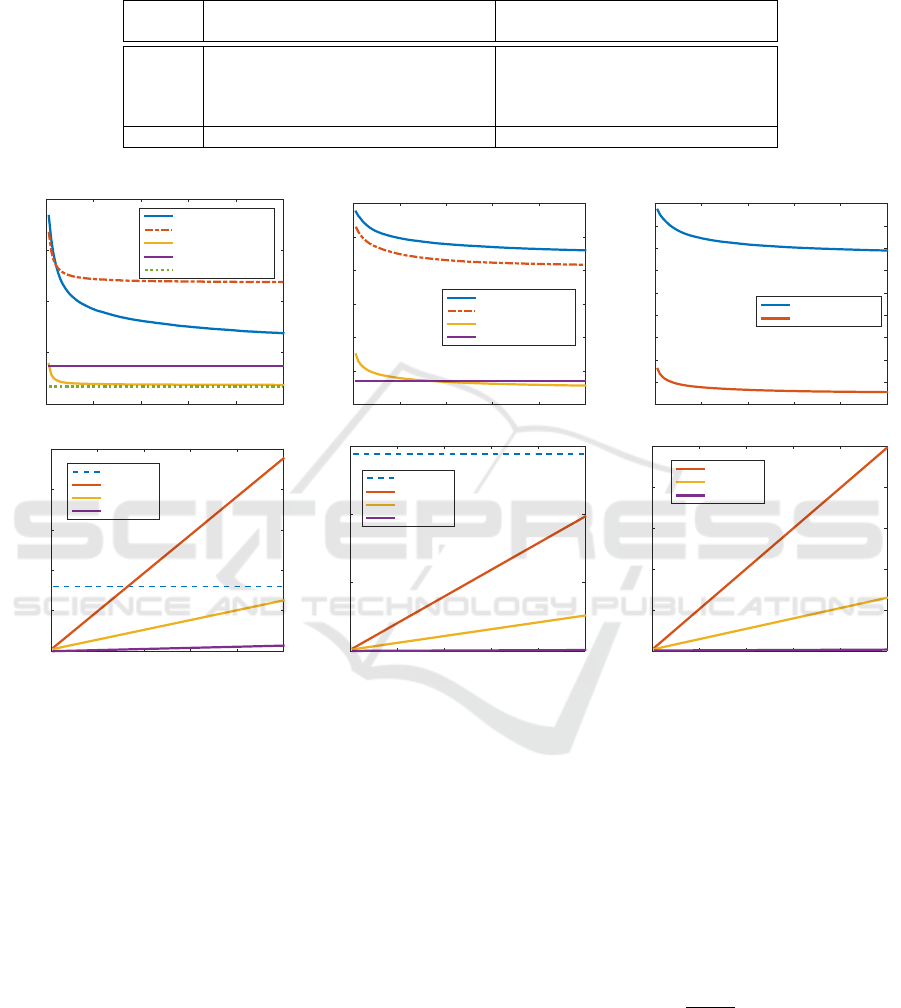
Table 1: Maximum, minimum, mean and standard deviation of the number K of optimal solutions reached by Uno’s Algo-

rithm. The procedure has been stopped at 10,000 optimal bipartite mappings at the most, implying that these results are not

representative of the whole set of optimal bipartite solutions, which is even bigger. The bipartite cost matrix computation

schemes are (Riesen and Bunke, 2009) and (Ga

ere et al., 2014).

Dataset

(Riesen and Bunke, 2009) (Ga

ere et al., 2014)

max(K) min(K)

K σ(K) max(K) min(K)

K σ(K)

Alkane 10000 1 6198 3847 10000 1 993 1977

Acyclic 10000 1 2313 3496 10000 1 182 857

MAO 10000 48 7695 3711 10000 1 948 2714

PAH 10000 10000 10000 0 10000 128 9894 879

CMU 16 1 1.6 1.5 -

a. Acyclic b. PAH c. MUTA

Number of solutions to LSAP

0 20 40 60 80 100

Mean approximate GED

Bunke

Random Walks

mIPFPE init Bunke

GNCCP (18.7)

A* (16.727)

Number of solutions to LSAP

0 20 40 60 80 100

Mean approximate GED

100

120

140

Bunke

Random Walks

mIPFPE init Bunke

GNCCP (34.2)

Number of solutions to LSAP

0 20 40 60 80 100

Mean approximate GED

120

130

140

150

160

170

180

190

200

210

Bunke

mIPFP init Bunke

Number of solution to LSAP

0 20 40 60 80 100

Mean Accumul. Computation time (s)

0.2

0.4

0.6

0.8

GNCCP

mIPFP seq

mIPFP mt

Init.

Number of solution to LSAP

0 20 40 60 80 100

Mean Accumul. Computation time (s)

GNCCP

mIPFP seq

mIPFP mt

Init.

Number of solution to LSAP

0 20 40 60 80 100

Mean Accumul. Computation time (s)

mIPFP seq

mIPFP mt

Init.

d. Acyclic e. PAH f. MUTA

Figure 1: Approximate GED (a., b. and c.) and computation times of IPFP against GNCCP (d., e. and f.) sequential (seq)

and multi-threaded (mt) implementations, in accordance with the number of initial mappings. The exact GED (A

∗

) is known

for Acyclic, and GNCCP could not be applied on MUTA because of its high time complexity.

standard library, as well as low-cost, sub-optimal, bi-

partite assignments which approximate the ones of

(Riesen and Bunke, 2009), obtained via a greedy al-

gorithm. These bipartite methods correspond to the

three kinds of initialization described in section 3 and

their results are given in the ﬁrst part of Table 2.

The quadratic approaches (second part of this ta-

ble) present a set of versions of IPFP and their ex-

tended mIPFP versions along with a convex-concave

procedure, GNCCP (Liu and Qiao, 2014), described

for GED estimation in (Bougleux et al., 2017) since

it uses a global search strategy which iterates in-

stances of IPFP algorithm. We complete this set of

experiments with the method of (Neuhaus and Bunke,

2007) which aims at resolving a relaxed version of

the quadratic assignment problem with classical opti-

mization tools.

The IPFP versions differ by their initializations

or sets of initial mappings. These sets are those de-

scribed in section 3. In addition, we also consider the

continuous initial vector j of same structure as matri-

ces in D

n,m,ε

, so that each coefﬁcient unconstrained to

be null is deﬁned by:

k,l

n+m+2

(12)

Flat initial vectors are used as an initialization of

the Frank-Wolfe algorithm in several works to be-

gin with a centered candidate solution. In Ta-

ble 2, IPFP

INIT

refers to the IPFP method (sec-

tion 2) initialized with a discrete or continuous so-

lution x ∈ S

INIT

= S

INIT

k=1

, where S

INIT

is a set of k so-

ICPRAM 2018 - 7th International Conference on Pattern Recognition Applications and Methods

154

Table 2: Mean approximate graph edit distance (d), error (e) and computation time in seconds (t), with a number of initial

assignments k = 40 on GREYC’s chemistry datasets. Nomenclature : bipartite estimation (bGED), IPFP quadratic estimation

(IPFP), m stands for multiple version, and r stands for recentered version

Algorithm

Alkane Acyclic MAO PAH

d e t d e t d t d t

A* 15.3 16.7

Bipartite

bGED Rie. and Bun. (2009) 37.8 22.5 ≈ 10

−4

33.3 16.6 ≈ 10

−4

95.7 10

−3

135.2 10

−3

bGED Ga

u. et al (2014) 36.0 20.7 0.02 31.8 15.0 0.02 85.1 1.48 125.8 2.60

mbGED Rie. and Bun. (2009) 25.5 10.2 0.01 23.1 6.4 0.01 75.1 0.05 116.0 0.02

mbGED Ga

u. et al (2014) 26.0 10.6 0.03 27.0 10.3 0.02 76.0 1.50 105.8 2.65

mbGED Random 60.2 44.9 ≈ 10

−4

52.6 35.8 ≈ 10

−4

164.3 ≈ 10

−4

194.1 ≈ 10

−4

mbGED Greedy 39.0 23.6 ≈ 10

−4

38.1 20.7 ≈ 10

−4

99.6 < 10

−3

135.7 < 10

−3

Frank-Wolfe

IPFP

Flat uniform init.

18.6 3.2 0.02 20.0 3.3 0.01 45.8 0.1 50.7 0.25

IPFP

Init. Rie. and Bun. (2009)

18.1 2.7 0.02 18.9 2.1 0.009 38.4 0.04 50.0 0.09

IPFP

Init. Ga

u. et al (2014)

18.0 2.7 0.04 18.7 2.1 0.02 38.7 1.53 46.8 2.68

IPFP

Random init.

19.9 4.6 0.02 22.2 5.4 0.01 56.3 0.07 53.2 0.10

IPFP

Random bistoch. init.

19.3 3.9 0.03 19.8 3.1 0.04 51.9 0.32 51.8 0.48

IPFP

Greedy init.

18.1 2.8 0.02 18.8 2.1 0.01 38.8 0.02 50.3 0.03

mIPFP

Init. Rie. and Bun. (2009)

15.4 0.07 0.20 16.9 0.2 0.10 31.4 0.48 33.6 1.10

mIPFP

Init. Ga

u. et al (2014)

15.6 0.20 0.18 17.4 0.7 0.08 33.4 1.75 30.5 3.58

mIPFP

Random init.

15.3 0.01 0.22 16.74 <0.01 0.13 33.3 0.81 36.6 1.17

mIPFP

Random bistoch. init.

15.3 0.01 0.20 16.73 <0.01 0.13 31.6 1.60 34.8 2.94

mIPFP

Greedy init.

15.4 0.06 0.17 16.8 0.03 0.11 31.8 0.46 35.4 1.01

Frank-Wolfe recentered

rIPFP

Init. Rie. and Bun. (2009)

17.9 2.5 0.03 18.7 2.0 0.03 38.5 0.14 48.3 0.18

rIPFP

Init. Ga

u. et al (2014)

17.7 2.4 0.07 18.7 2.0 0.05 35.8 1.63 45.3 2.73

rIPFP

Random init.

18.2 2.9 0.04 19.1 2.4 0.03 45.9 0.15 50.6 0.19

rIPFP

Random bistoch. init.

18.2 2.9 0.03 19.0 2.3 0.03 45.0 0.15 50.7 0.19

rIPFP

Greedy init.

17.8 2.5 0.04 18.6 1.9 0.03 38.7 0.14 48.0 0.18

rmIPFP

Init. Rie. and Bun. (2009)

15.4 0.12 0.09 16.8 0.1 0.07 31.37 0.40 31.5 0.70

rmIPFP

Init. Ga

u. et al (2014)

15.5 0.21 0.15 17.2 0.4 0.09 32.40 1.75 29.8 2.96

rmIPFP

Random init.

15.3 0.03 0.10 16.74 0.02 0.07 31.40 0.48 32.8 0.75

rmIPFP

Random bistoch. init.

15.3 0.04 0.10 16.75 0.03 0.07 31.42 0.44 32.8 0.74

rmIPFP

Greedy init.

15.4 0.08 0.10 16.75 0.03 0.08 31.39 0.48 32.4 0.75

GNCCP 16.6 1.2 0.58 18.7 1.3 0.32 34.3 9.23 34.2 14.44

Neuhaus and Bunke (2007) 20.5 - 0.07 25.7 - 0.04 59.1 7.0 52.9 8.2

lutions corresponding to INIT. mIPFP then refers to

mIPFP(∆,S

INIT

), the multistart version of IPFP that

is, IPFP

INIT

stands for mIPFP(∆,S

INIT

). Finally, we

consider initializations re-centered in the continuous

space from an initial x

∈ S

INIT

x =

+ j) (13)

These re-centered versions are denoted by rIPFP and

rmIPFP in Table 2. The sequential and parallel ver-

sions of mIPFP are both implemented, but the times

given in the tables refer to the multi-threaded variant

with at most 4 threads.

Datasets. We performed our experiments on 5

chemoinformatics datasets

and a geometric one.

The chemistry data are symbolic graphs represent-

ing molecules. Nodes correspond to atoms and edges

Available at https://iapr-tc15.greyc.fr/links.html

are valence bounds. There are four different types of

graphs : acyclic unlabeled (Alkane), acyclic labeled

(Acyclic), unlabeled (PAH) and labeled (MAO). The

ﬁfth chemistry dataset MUTA (Riesen and Bunke,

2008), is originally separated into seven subsets by

molecule size, from 10 to 70 atoms. In our experi-

ments, we randomly selected a subset of 100 graphs

over all the molecule sizes in MUTA, to let insertions

and deletions play an appreciable role, which is not

the case when the graph size is ﬁxed

The Geometric graphs of CMU (Riesen and

Bunke, 2008) represent 30 points of interest manu-

ally picked up over a series of images depicting a

toy house captured from different viewpoints. Nodes

are labeled according to the coordinates of the points

(precision of 10

−6

) and edge labels are the euclidean

distance between them. Note that the GED-estimation

method of (Ga

ere et al., 2016) needs the data to

be integer typed, hence it could not be applied to the

Approximate Graph Edit Distance by Several Local Searches in Parallel

155

CMU datasets in our experiments. The graph pairs we

tested on this dataset are the same as in (Abu-Aisheh

et al., 2015).

Table 3: Mean approximate graph edit distance (d), error

(e) and computation time (t), with a number of initial as-

signments k = 40. Datasets MUTA and CMU.

Algorithm

MUTA CMU k = 16

d t d t

bGED R. and B. 209 0.02 1810 0.01

mbGED R. and B. 196 0.9 1791 0.10

mbGED Random 276 < 10

−3

> 10

< 10

−3

mbGED Greedy 210 0.005 4418 0.02

IPFP

Init. R. and B.

136 0.07 410 0.07

IPFP

Random init.

142 0.1 6532 0.90

IPFP

Init. Greedy

136 0.09 414 0.02

mIPFP

Init. R. and B.

127 3.25 410 1.35

mIPFP

Random init.

128 5.20 472 13.64

mIPFP

Init. Greedy

133 3.58 415 0.7

GNCCP - 408 6.66

Analysis. Table 1 presents statistical information

about the number of optimal solutions of the LSAP

reached by Uno’s algorithm for each dataset. In order

to keep a reasonable computation time, we bounded

the algorithm by K

max

= 10

mappings. One can see

that the number of these optimal assignments can be

huge for symbolic graphs. These graphs, and in par-

ticular unlabeled graphs, lead indeed to relatively ﬂat

linear cost matrices. The corresponding LSAP have

then a large number of optima. In contrast, the geo-

metric dataset CMU presents not much optimal solu-

tions with at most 16 ones, and generally 1 to 2 opti-

mal assignments per graph pair. These results shows

that on symbolic graphs, the strategy of taking an ar-

bitrary optimal bipartite solution to approximate the

GED can legitimately be questioned, as there can be

thousands of them.

Among the one-shot approaches, the bipartite ap-

proximation (Riesen and Bunke, 2009) gives esti-

mations which are far higher than the quadratic ap-

proaches (IPFP, GNCCP and Neuhaus and Bunke).

The gap deepens when the graph’s size increases, but

even small graphs of Alkane and Acyclic give error

rates 6 to 7 times higher than the reﬁned assignments.

The extended version mbGED allows the estima-

tion to decrease rapidly depending on the number of

considered optimal assignments (see ﬁgure 1 a. b.

c.). We made this observation over all the consid-

ered datasets, especially for symbolic labeled data.

We can deduce that there are indeed better optimal bi-

partite assignments than the arbitrary ones, and more-

over, the gain in term of precision considering them

is signiﬁcant, up to halve the error on some datasets

as shown in table 2. This highlights that in the con-

text of bipartite approximation, it is needed to search

not only for an optimal assignment, but also a rele-

vant one to estimate the GED. However, even consid-

ering 100 assignments, the bipartite estimations are

still above the quadratic ones.

While the Random-Walk based method to design

the bipartite cost matrix (Ga

ere et al., 2014) tends

to give better approximations with k = 1, it stabi-

lizes quicker when considering several assignments

on small sized graphs. Our interpretation of this is

that the downsized set of optimal solutions available

leads to less good ones in the context of GED estima-

tion, thus a faster convergence. More, the length of

the walks, here set to 3, is large in comparison to the

diameter of the small graphs, so they don’t allow to

represent well the neighborhoods, hence this method

is more relevant on larger graphs. Notice that the high

computation time required here comes from the deter-

mination of the cost matrix, and not from the compu-

tation of the k − 1 remaining optimal mappings.

Compared to LSAP approaches, IPFP improves

dramatically the accuracy of GED estimations. How-

ever, as stated in subsection 2, this algorithm needs to

be initialized, and the initialization choice impacts a

lot on the obtained approximation. This is illustrated

in tables 2 and 3. Apart from the random initializa-

tions, all discrete initial vectors we tested lead to bet-

ter estimations than the trivial ﬂat uniform continuous

vector j. Indeed, initial vectors which are close to low

local minima of the quadratic function Q(x, ∆) will

lead to lower results in a smaller number of iterations.

In term of time complexity, IPFP will need more iter-

ations to converge from an initial value farther from a

local minimum, as we can remark in the case of ran-

dom initializations. This behavior deepens with the

multistart version mIPFP, as it is about iterating sev-

eral times this algorithm.

GNCCP estimation is more precise than single-

start IPFP on all tested datasets, as each iteration gives

a better initialization to the next. An advantage of this

method is that it does not need an initial guess, be-

cause the ﬁrst iteration resolves a fully convex prob-

lem. However, the amount of time needed to reach the

global minimum during this ﬁrst iteration could be re-

duced with a relevant initial assignment. Moreover, if

the ﬁrst IPFP call needs too much time to converge,

it can be stopped in the implementation by reaching

the maximum number of iterations, thus leading to a

less relevant initialization to the next IPFP call and so

on. Yet, an initialization step for GNCCP is not part

of this paper and could be studied in a future work.

Such as IPFP, mIPFP is strongly impacted by its

initialization set, especially in term of computation

ICPRAM 2018 - 7th International Conference on Pattern Recognition Applications and Methods

156

time. Considering the approximation, mIPFP is the

more accurate method on all the tested datasets, CMU

excepted. Still, there is no initialization method that

beats the others on all the datasets. Good results have

been obtained via random initial assignments, which

can seems surprising while each IPFP may converge

to a far-from-optimal local minimum. But consider-

ing the fact that initial assignments should lie far from

each others in order to get different estimation of the

GED (i.e. generate few collisions through the IPFP

process), randomly generated initial guesses may sat-

isfy this condition. Nevertheless, each randomly ini-

tialized IPFP needs generally more time to converge,

since an initial assignment has a relatively low proba-

bility to be close to a local minimum.

mIPFP beats GNCCP over all the symbolic

datasets, with several kind of initializations. We be-

lieve that this result is related to the fact that one iter-

ation of GNCCP needs more IPFP iterations to con-

verge, and as many more as the treated problem is

convex or concave. We noticed that the total num-

ber of IPFP iteration through the GNCCP procedure is

frequently far higher to the total number of IPFP iter-

ations in the sequential mIPFP process (with k = 40).

As the number of iterations is bounded, a GNCCP it-

eration may not terminate on a close-to-optimal value,

in particular in the convex situation, and this has an

impact on the forthcoming iterations thus restraining

the convergence of GNCCP. Moreover, a higher num-

ber of IPFP iterations for GNCCP leads to a higher

computation time.

Finally, the re-centering procedure enhances a lit-

tle the reﬁned solutions, in particular concerning large

graphs. The gain achieved with respect to the graph

size begins to be signiﬁcant with the dataset PAH. We

also noticed a reduction of the needed time with these

graphs, and these results should be subjected to fur-

ther experiments on larger graphs.

5 CONCLUSIONS AND FUTURE

WORK

In this paper, we propose to reﬁne bipartite GED with

multiple-initialized IPFP. We show that this simple

idea constitutes an alternative to more sophisticated

procedures like GNCCP, with the advantage to be eas-

ily parallelized. We study the impact of initialization

on this method through three kinds of assignments :

randomly generated, low-cost, and optimal bipartite

assignments. We show that our results with these

strategies are relatively close to each other, and com-

pete with stat-of-the art methods for estimating the

GED with a lower computation time.

In future work, we plan to seek how to get more

relevant sets of initializations to mIPFP, considering

a distance between assignments or by guiding their

enumeration by the quadratic costs. Another axis of

consideration is to study a possible way of initializing

GNCCP to get more precise estimations, in a better

time complexity.

REFERENCES

Abu-Aisheh, Z., Ga

uzere, B., Bougleux, S., Ramel, J.-Y.,

Brun, L., Raveaux, R., H

eroux, P., and Adam, S.

(2017). Graph edit distance contest: Results and fu-

ture challenges. Pattern Recognition Letters, 100:96–

103.

Abu-Aisheh, Z., Raveaux, R., and Ramel, J.-Y. (2015). A

graph database repository and performance evaluation

metrics for graph edit distance. In IAPR Internatioanl

workshop on Graph Based Representation.

Blumenthal, D. B. and Gamper, J. (2017). Exact com-

putation of graph edit distance for uniform and non-

uniform metric edit costs. In Graph-Based Repre-

sentations in Pattern Recognition, volume 10310 of

LNCS, pages 211–221.

Bougleux, S., Brun, L., Carletti, V., Foggia, P., Ga

ere,

B., and Vento, M. (2017). Graph edit distance as a

quadratic assignment problem. Pattern Recognition

Letters, 87:38–46.

Bunke, H. and Allermann, G. (1983). Inexact graph match-

ing for structural pattern recognition. Pattern Recog-

nition Letters, 1(4):245–253.

Burkard, R., Dell’Amico, M., and Martello, S. (2009). As-

signment Problems. SIAM.

Cappellini, V., Sommers, H.-J., Bruzda, W., and

Zyczkowski, K. (2009). Random bistochastic matri-

ces. Journal of Physics A: Mathematical and Theoret-

ical, 42(36):365209.

Carletti, V., Ga

ere, B., Brun, L., and Vento, M. (2015).

Approximate graph edit distance computation com-

bining bipartite matching and exact neighborhood

substructure distance. In Graph-Based Representa-

tions in Pattern Recognition, volume 9069 of LNCS,

pages 168–177.

Cort

es, X., Serratosa, F., and Moreno-Garc

ıa, C. F. (2015).

On the inﬂuence of node centralities on graph edit dis-

tance for graph classiﬁcation. In Int. Workshop on

Graph-Based Representations in Pattern Recognition,

volume 9069 of LNCS, pages 231–241. Springer Int.

Pub.

Fischer, A., Riesen, K., and Bunke, H. (2017). Improved

quadratic time approximation of graph edit distance

by combining hausdorff matching and greedy assign-

ment. Pattern Recognition Letters, 87:55–62.

Frank, M. and Wolfe, P. (1956). An algorithm for quadratic

programming. Naval Research Logistics Quarterly,

3(1-2):95–110.

ere, B., Bougleux, S., and Brun, L. (2016). Approx-

imating graph edit distance using GNCCP. In Struc-

Approximate Graph Edit Distance by Several Local Searches in Parallel

157

tural, Syntactic, and Statistical Pattern Recognition,

volume 10029 of LNCS, pages 496–506. Springer Int.

Pub.

ere, B., Bougleux, S., Riesen, K., and Brun, L. (2014).

Approximate graph edit distance guided by bipartite

matching of bags of walks. In Structural, Syntactic,

and Statistical Pattern Recognition, volume 8621 of

LNCS, pages 73–82.

Knight, P. A. (2008). The Sinkhorn-Knopp algorithm: Con-

vergence and applications. SIAM Journal on Matrix

Analysis and Applications, 30(1):261–275.

Lawler, E. (1963). The quadratic assignment problem.

Management Sci., 9:586–599.

Leordeanu, M., Hebert, M., and Sukthankar, R. (2009). An

integer projected ﬁxed point method for graph match-

ing and map inference. In Advances in Neural Infor-

mation Processing Systems, volume 22, pages 1114–

1122.

Lerouge, J., Abu-Aisheh, Z., Raveaux, R., H

eroux, P., and

Adam, S. (2017). New binary linear programming for-

mulation to compute the graph edit distance. Pattern

Recognition, 72:254–265.

Liu, Z.-Y. and Qiao, H. (2014). GNCCP–Graduated

NonConvexity and Concavity Procedure. IEEE

Trans. on Pattern Analysis and Machine Intelligence,

36(6):1258–1267.

Neuhaus, M. and Bunke, H. (2007). Bridging the Gap Be-

tween Graph Edit Distance and Kernel Machines, vol-

ume 68 of Machine Perception and Artiﬁcial Intelli-

gence. World Scientiﬁc Publishing Co., Inc.

Riesen, K. (2015). Structural Pattern Recognition with

Graph Edit Distance. Advances in Computer Vision

and Pattern Recognition. Springer Int. Pub.

Riesen, K. and Bunke, H. (2008). IAM graph database

repository for graph based pattern recognition and

machine learning. accepted for publication in SSPR

2008.

Riesen, K. and Bunke, H. (2009). Approximate graph

edit distance computation by means of bipartite graph

matching. Image and Vision Computing, 27:950–959.

Riesen, K. and Bunke, H. (2015). Improving bipar-

tite graph edit distance approximation using various

search strategies. Pattern Recognition, 28(4):1349–

1363.

Riesen, K., Bunke, H., and Fischer, A. (2014). Improv-

ing graph edit distance approximation by centrality

measures. In Int. Conf. on Pattern Recognition, pages

3910–3914.

Riesen, K., Ferrer, M., Fischer, A., and Bunke, H. (2015).

Approximation of graph edit distance in quadratic

time. In Int. Workshop on Graph-Based Representa-

tions in Pattern Recognition, volume 9069 of LNCS,

pages 3–12. Springer Int. Pub.

Riesen, K., Fischer, A., and Bunke, H. (2017). Improved

graph edit distance approximation with simulated an-

nealing. In Graph-Based Representations in Pattern

Recognition, volume 10310 of LNCS, pages 222–231.

Springer International Publishing.

Sanfeliu, A. and Fu, K.-S. (1983). A distance measure be-

tween attributed relational graphs for pattern recogni-

tion. IEEE Transactions on Systems, Man. and Cyber-

netics, 13(3):353–362.

Serratosa, F. (2014). Fast computation of bipartite graph

matching. Pattern Recognition Letters, 45:244–250.

Serratosa, F. (2015). Computation of graph edit distance:

Reasoning about optimality and speed-up. Image and

Vision Computing, 40:38–48.

Sinkhorn, R. and Knopp, P. (1967). Concerning nonnega-

tive matrices and doubly stochastic matrices. Paciﬁc

Journal of Mathematics, 21(2):343–348.

Uno, T. (1997). Algorithms for enumerating all per-

fect, maximum and maximal matchings in bipartite

graphs. In Algorithms and Computation, volume 1350

of LNCS, pages 92–101. Springer Verlag.

Vogelstein, J. T., Conroy, J. M., Lyzinski, V., Podrazik, L. J.,

Kratzer, S. G., Harley, E. T., Fishkind, D. E., Vogel-

stein, R. J., and Priebe, C. E. (2015). Fast approximate

quadratic programming for graph matching. PLOS

ONE, 10(4):1–17.

Zaslavskiy, M., Bach, F., and Vert, J.-P. (2009). A path

following algorithm for the graph matching problem.

Pattern Anal. Mach. Intell., 31(12):2227–2242.

Zeng, Z., Tung, A. K. H., Wang, J., Feng, J., and Zhou,

L. (2009). Comparing stars: On approximating graph

edit distance. Proceedings of the VLDB Endowment,

2(1):25–36.

ICPRAM 2018 - 7th International Conference on Pattern Recognition Applications and Methods

158