Whole Day Mobility Planning with Electric Vehicles
Marek Cuch
´
y, Michal
ˇ
Stolba and Michal Jakob
Artificial Intelligence Center, Faculty of Electrical Engineering,
Czech Technical University in Prague, Czech Republic
Keywords:
Electric Vehicles, Mobility Planning, Charging, Speed-Ups, Road Networks.
Abstract:
We propose a novel and challenging variant of trip planning problems – Whole Day Mobility Planning with
Electric Vehicles (WDMEV). WDMEV combines several concerns, which has been so far only considered
separately, in order to realistically model the problem of planning mobility with electric vehicles (EVs). A key
difference between trip planning for combustion engine cars and trip planning for EVs is the comparatively
lower battery capacity and comparatively long charging times of EVs – which makes it important to carefully
consider charging when planning travel. The key idea behind WDMEV is that the user can better optimize
his/her mobility with EVs, if it considers the activities he/she needs to perform and the travel required to get to
the locations of these activities for the whole day - rather than planning for single trips only. In this paper, we
formalize the WDMEV problem and propose a solution based on a label-setting heuristic search algorithm,
including several speed-ups. We evaluate the proposed algorithm on a realistic set of benchmark problems,
confirming that the whole day approach reduces the time required to complete one’s day travel with EVs and
that it also makes it cheaper, compared to the traditional single-trip approach.
1 INTRODUCTION
One of the most prominent drawbacks of the use of
Electric Vehicles (EVs) is the range anxiety and long
charging times. An average EV can travel about 150-
200km on a fully charged battery, whereas charging the
battery for the average range of 150 kilometers takes
about 4-12 hours using a slow-charging technology
(e.g., home outlet) and about 30 minutes using a fast-
charging technology (e.g., CHAdeMO). EV users need
to plan their trips so that they do not run out of battery
mid-way; if charging is necessary, they need to plan it
carefully so that charging does not delay their activities
and they arrive for their duties on-time.
Although there is a wealth of literature on path
planning with energy constraints and charging and re-
lated problems, the existing solutions focus on isolated
planning of single trips and do not take into account
the whole day context of mobility. In this work we
propose to take a more holistic perspective, where
we take into account not only the route planning and
charging, but also the temporally and spatially con-
strained activities which need to be performed by the
users. By taking the whole day activity and mobility
model into consideration, our approach provides better
solutions compared to single-trip planners that handle
each requests independently.
Take for example the scenario in Figure 1. The user
starts and ends in the home location A, may charge
the EV at B and D and shop at B. The user’s goal is
to spend 8 hours at the workplace and to shop for 30
minutes. The initial (and maximal) capacity of the
EV battery is 30 kWh and charging to full takes 60
minutes. In the naive plan shown in Figure 1a), the
user first decides the order of activities, that is, first go
to work and then do the shopping. Also the charging is
postponed until necessary. By this approach, the user
first goes to location C (the EV has enough charge to
do that) and works for 8 hours. Next, the user wants to
go home and make a stop for shopping. However the
charge of the EV is not high enough to do so, and thus
the user must first go to a nearby charging station at
location C. Then the user can get to location B and do
the shopping while also charging the EV. At the end,
when the user gets home, the time overhead caused by
charging is 45 minutes (we do not count the charging
time while shopping).
By optimizing for the whole day formulation of
the problem, the user can obtain the optimized plan
shown in Figure 1b), where the shopping is scheduled
before work. In that case, the user first arrives at
B, does the shopping while recharging the battery to
full and continues to work. On the way back, the
EV does not have enough charge for the whole trip
154
Cuchý, M., Štolba, M. and Jakob, M.
Whole Day Mobility Planning with Electric Vehicles.
DOI: 10.5220/0006598501540164
In Proceedings of the 10th International Conference on Agents and Artificial Intelligence (ICAART 2018) - Volume 2, pages 154-164
ISBN: 978-989-758-275-2
Copyright © 2018 by SCITEPRESS – Science and Technology Publications, Lda. All rights reserved

A
B C D
1h
15kWh
30min
10kWh
5min
5kWh
7:00
30 kWh
8:00
15 kWh
16:30
5 kWh
work (8h)
8:30
5 kWh
16:35
0 kWh
charge (15 kWh)
17:05
15 kWh
17:10
10 kWh
17:40
0 kWh
shop (30min)
charge (15 kWh)
18:10
15 kWh
19:10
0 kWh
A
B C D
1h
15kWh
30min
10kWh
5min
5kWh
7:00
30 kWh
8:00
15 kWh
work (8h)
9:00
20 kWh
charge (5 kWh)
17:40
15 kWh
17:30
10 kWh
shop (30min)
charge (15 kWh)
8:30
30 kWh
18:40
0 kWh
17:00
20 kWh
a) b)
Figure 1: Example scenario: A - home location, C - work location, B, D - chargers, B - shop. Activities are 8h work, 30min
shop. Maximal state of charge (SOC) - 30 kWh, charging to full takes 60 minutes. a) Naive approach: The user first decides
the order of activities (work, shop). Charging postponed until necessary. b) Whole day formulation: Optimize the order of
activities and charging (shop,work).
and thus a short (10 min) charging stop is scheduled.
Overall, the user arrives 30 minutes earlier than in the
naive case and spends only 10 minutes on charging
overhead. Notice also that the total energy consumed
from charging stations is 10 kWh less which might
also save money.
Obviously, this simple problem is easy to optimize,
but the problem gets too complicated for a human
when the number of locations and activities increases
and the temporal constraints get more complicated.
Informally, the Whole Day Mobility Planning with
Electric Vehicles (WDMEV) problem can be modeled
as a search problem on a road network graph with
specific vertices being charging stations and points of
interest (POIs) where given activities can be performed
in given time windows. Each edge in the graph (corre-
sponding to road segments) has a particular time cost
depending on the distance and maximal speed (we do
not allow choosing the cruise speed) and energy cost
depending mainly on the elevation profile (as the EV
can recuperate energy when going downhill) and the
speed.
Each of the activities the user wants to perform is
associated with a particular location and is constrained
by the earliest activity start time (the time when the
activity can be started at the earliest), the latest activity
end time, that is, the time when the activity must be
finished at the latest, and the activity duration which
is fixed. This gives us a time window in which the
activity duration must fit. Each charging station is as-
sociated with a location, cost of charging per minute,
and charging speed depending on the technology avail-
able at the charging station. The cost of charging can
differ between the charging stations but is considered
to be constant throughout the time (as is the case at
most current charging stations). We are interested in
minimizing the total time spent traveling and perform-
ing activities, the total money cost of the trip (where
the money is spent on charging stations), or both at the
same time.
The main challenges of solving the proposed prob-
lem are the following. The underlying Traveling Sales-
man Problem (TSP) makes the whole problem NP-
hard (Krentel, 1988). However as was shown in the
example, sequencing the activities up-front may sig-
nificantly reduce the quality of the solution, or even
make the problem unsolvable. This is mainly due to
the temporal constraints which may be not satisfiable
in some orderings. Another source of complexity is
a limited capacity of batteries (and thus limited range
of autonomy of the EV). The state of charge (SOC)
of the battery must be taken into account during the
optimization in order to ensure that a path worse ac-
cording to the selected metric (e.g., time) but with a
higher SOC is not discarded as this might lead to a so-
lution whereas the better path might end in a dead-end
(i.e., without enough SOC to reach the goal).
The contribution of this work is threefold:
• We formalize the novel Whole Day Mobility Plan-
ning with Electric Vehicles (WDMEV) problem.
• We propose a solution based on a label-setting
heuristic search algorithm, together with a number
of speed-ups.
• We experimentally analyze the algorithm and iden-
tify influences of the proposed heuristic and speed-
ups.
Whole Day Mobility Planning with Electric Vehicles
155

2 RELATED WORK
A large number of models and algorithms related to
particular sub-problems of the WDMEV problem have
been formulated in the literature. The basic problem
we can consider is the shortest-path problem on a graph
and the corresponding Dijkstra’s algorithm (Dijkstra,
1959). A multi-criteria version of the shortest path
problem together with a modification of the Dijkstra’s
algorithm was introduced in (Hansen, 1980). In the
multi-criteria version, the notion of the shortest path is
superseded with the idea of the set of Pareto-optimal
paths, that is, a set of paths which are not dominated
on all criteria by any other path. A generalization
of the Dijkstra’s algorithm leads to the label-setting
algorithm (Nemhauser, 1972) with arbitrary labels.
When considering EVs, the battery capacity and
charging become crucial. In (Khuller et al., 2011)
the authors present a number of gas station problems
(including shortest path and TSP) where the vehicle
has a limited tank capacity and can refuel at some
of the graph nodes with either a variable or uniform
price. The authors present a number of dynamic pro-
gramming solutions and approximations. In (Artmeier
et al., 2010; Sachenbacher et al., 2011) the authors
study energy-optimal routing for electric vehicles by
first casting it as a variant of the Constrained Shortest
Path Problem (CSPP) (Beasley and Christofides, 1989)
with an O(n
3
) algorithm, and second by solving it as a
graph search problem with the A* (Hart et al., 1968)
algorithm and a consistent heuristic yielding an O(n
2
)
solution.
In practice, the EV routing problem is also solved
by various commercial
1
and academic routing ser-
vices (Fi
ˇ
ser, 2017). The battery limit and charging
is often considered not only for the single shortest path
problem but also for TSP or VRP problems. In (Felipe
et al., 2014) the authors consider the case of routing
a fleet of vehicles as a Green Vehicle Routing Prob-
lem (GVRP), with multiple modes of recharging (as
in our case) but without the temporal constraints. The
Electric Vehicle Routing Problem (EVRP) with time
windows solved in (Desaulniers et al., 2016; Schneider
et al., 2014) is the closest fit to the WDMEV problem
considered in our work. In contrast to the EVRP, our
approach focuses on single vehicle routing with pos-
sible future extensions to time-dependent costs (both
the time of driving and the cost of charging) and multi-
criteria optimization (the label-setting algorithm can
be easily modified for such a case). Moreover, our ap-
proach is based on an optimal algorithm and also most
of proposed speed-ups preserve optimality. In (Arslan
1
http://www.evjourney.com;
https://abetterrouteplanner.com; https://www.egomap.eu
et al., 2015) the authors have shown that the mini-
mal cost path problem for EVs (or for Hybrid Plug-in
EVs in their case) is NP-hard by transforming it to the
Shortest Weight-Constrained Path Problem (SWCPP)
which was shown to be NP-hard in (Garey and John-
son, 2002).
Another important facet of our Whole Day Mobil-
ity Planning with Electric Vehicles (WDMEV) prob-
lem is time. Again, there are many temporal exten-
sions of the individual sub-problems. The Shortest
Path Problem with Time Windows (SPPTW) has been
solved with a label-setting algorithm in (Desrochers
and Soumis, 1988) and an optimal algorithm based on
dynamic programming has been proposed by (Ioachim
et al., 1998). A summary of time-constrained
vehicle routing and scheduling problems (includ-
ing TSP) and respective algorithms was published
in (Desrosiers et al., 1995). An optimal algorithm
was presented in (Dumas et al., 1995) and an approxi-
mation in (Bansal et al., 2004).
In our case, the combination of time windows on
the locations to visit and resources consumed on the
edges (but also replenished at some locations) needs
to be considered. A very recent work (Veneti et al.,
2016) have considered a closely related problem in
the sea transportation domain. The authors propose a
special case of Time-Dependent Shortest Path Prob-
lem (TDSPP) where the path must visit a specified
sequence of nodes and also a TSP variant, both includ-
ing bi-criteria optimization. The particular criteria are
fuel consumption and safety. In addition to temporal
constraints in the ports to visit, the properties (e.g.,
cost) of the graph change in time depending mainly on
the weather situation. Closely related is also the Trip
Query Problem (TQP) (Li et al., 2005) which consists
of the problem of planning a trip over points of inter-
est such that each belongs to a specific category and
at least one point of interest from each category has
to be visited, also studied as generalized TSP (Rice
and Tsotras, 2013). A temporal extension of a similar
problem (Multi-Type Nearest Neighbor) was studied
in (Ma et al., 2009). In our current problem, we do
not consider multiple locations for each activity. In-
stead , we focus on the temporal and SOC constraints
which, to our best knowledge, have not been studied
in combination yet.
3 PROBLEM DEFINITION
In this section we propose a formal definition of the
WDMEV problem. Let G = (V,E) be a directed graph
representing the underlying road network, where V
is a set of vertices and E is a set of edges and each
ICAART 2018 - 10th International Conference on Agents and Artificial Intelligence
156

edge (u,v) ∈ E is associated with two cost attributes,
a non-negative time cost tc(u,v) and an energy cost
ec(u,v), which can be negative due to recuperation.
Let C ⊆ V be a set of charging stations where each
charging station c ∈ C has a set of available charging
rates P
c
⊆ P and charging costs per time unit of charg-
ing cc
c
(ρ) for each charging rate ρ ∈ P
c
. P is a set
of all possible charging rates. The time required for
charging is the function
ct : P× [0,β
max
) × (0, β
max
] → N
+
mapping a charging rate, an initial SOC and a final
SOC on the charging time. β
max
∈ R
+
is the maxi-
mal state of charge. Besides the maximal β
max
we
define the minimal state of charge β
min
below which
the battery should not drop at any point in the plan.
This parameter represents the need of drivers to keep
some energy reserve. Otherwise the inaccuracy of the
consumption estimates may lead to a fully depleted
battery during the plan execution even though in the
plan the SOC was not expected to drop below 0.
Let A ⊆ V be a set of activities to be planned. Each
activity a ∈ A is associated with the following time
constraints: EST(a) is the earliest start time, LET(a)
is the latest end time, and AD(a) is the activity dura-
tion which also implies the latest possible start time
LST(a) = LET(a) − AD(a).
The initial state of the problem is specified by the
starting location s ∈ V and an initial battery state of
charge β
init
.
The goal is to find a sequence of tuples π =
(hv
i
,τ
i
,β
i
,γ
i
i|i ∈ {1,...,k}) defining an order of the
visited nodes v
i
∈ V with the time τ
i
∈ N
0
, state of
charge β
i
∈ [β
min
,β
max
] and money cost of the γ
i
∈ R
+
0
such that the SOC never drops bellow allowed level
and all activities are performed ∀a ∈ A∃i ∈ {1, ..., k} :
v
i
= a∧EST(a) ≤ τ
i
≤ LST(a)∧v
i+1
= a∧τ
i+1
−τ
i
≥
AD(a) . Also the sequence has to start and end at the
initial location ( v
1
= v
k
= s ). The time and money
costs are non-decreasing ( ∀i, j ∈ {1, ...k} : i > j =⇒
τ
i
≥ τ
j
∧ γ
i
≥ γ
j
) but the SOC alters in both direction.
It can decrease by moving and increase due to the recu-
peration or charging. If the vehicle is charged it must
stay at the charging station while the SOC increases
- v
i
∈ C ∧ v
i+1
= v
i
∧ β
i+1
> β
i
. The properties of the
charging (cost, amount of energy recharged, etc.) can
be derived from the two consecutive states.
We consider the optimization metric of the WD-
MEV problem to be a weighted sum of the time and
money costs, formally
f (π) = w
τ
τ
k
+ w
γ
γ
k
where w
τ
,w
γ
∈ [0, 1] are the criteria weights. Nat-
urally, the problem can be cast as a multi-criteria op-
timization and the proposed solution would be easy
to modify. Nevertheless we leave this extension for
future work for simplicity of exposure.
4 SOLUTION APPROACH
Our solution is based on the idea of the label-setting
algorithm. The difference between the classic Dijk-
stra’s algorithm and the label-setting algorithm is that
instead of maintaining a single label for each opened
vertex, the label-setting algorithm maintains a Pareto
set L
v
of all non-dominated labels
l
v
= (A
vis
,τ,β,γ)
where A
vis
⊆ A is the set of activities already visited,
τ is the time required to get to state v , β is the current
SOC, and γ is the money cost of the path leading to
v respective to the label l
v
. In order to determine the
Pareto set L
v
, we use the following definition of the
dominance relation ≺.
Definition 1. Let l
v
,l
0
v
be two labels of the same node
v . We say that l
v
is dominated by l
0
v
(denoted as l
v
≺ l
0
v
)
iff the following conditions are satisfied:
A
vis
⊆ A
0
vis
f (τ,γ) ≥ f (τ
0
,γ
0
)
β ≥ β
0
(1)
where f (τ,γ) is the criteria function minimized by
the algorithm.
The pseudo-code of the proposed solution is shown
in Algorithm ?? . In each iteration of the algorithm, a
label l
v
of a vertex v ∈ V is polled from the priority
queue Q . The labeled state is expanded and the new
labels are added to the queue (Line 12). There are four
possible ways to expand the states, each representing
one action the user can do: (i) driving, (ii) performing
an activity, (iii) charging, and (iv) charging during an
activity. We distinguish between actions and activities
in the context of the search as activities are just one
type of actions of the user which also include driving
and charging. The four possible expansions are the
following:
(i) Driving Let v be the polled node and l
v
=
(A
vis
,τ,β,γ) the label currently being expanded.
For each outgoing edge (v, u) ∈ E, a new label
l
u
= (A
vis
,τ + tc(v, u), min(b − ec(v,u),β
max
),γ)
is added to the queue. The labels with the SOC
bellow β
min
are discarded.
(ii) Performing an activity An activity can be per-
formed iff the current location v is an activity loca-
tion ( v ∈ A ) and the activity has not been performed
Whole Day Mobility Planning with Electric Vehicles
157

Algorithm 1: Pseudo-code of the proposed WDMEV solu-
tion.
1 Algorithm plan()
2 Q: heap of labels l
v
= (A
vis
,τ,β,γ) ordered
by criteria function f and then by β
3 l
s
= (
/
0,0,β
init
,0) % initial label
4 Q ← {l
s
}
5 L
s
← {l
s
}
6 ∀v ∈ V \ {s} : L
v
←
/
0 % initialize the
Pareto-set for each node
7 while Q 6=
/
0 do
8 l
v
←extractMin(Q)
9 if isGoal(l
v
) then
10 return l
v
11 else
12 Q
0
←expand(l
v
)
13 Q
0
←prune(Q
0
)
14 forall the l
u
∈ Q
0
do
15 if @l
∗
u
∈ L
u
: l
u
≺ l
∗
u
then
16 Q ← Q \ {l
0
u
∈ L
u
|l
0
u
≺ l
u
}
17 Q ← Q ∪ {l
u
}
18 L
u
← L
u
\ {l
0
u
∈ L
u
|l
0
u
≺ l
u
}
19 L
u
← L
u
∪ {l
u
}
20 end
21 end
22 end
23 end
so far ( v /∈ A
vis
). The starting time τ
s
(implying
also the end time τ
e
= τ
s
+ AD(v) ) is set to the
earliest available moment ( τ
s
= max(τ,EST(v)) )
satisfying the activity time constraints. With time-
independent costs, a later start can never result into
a better solution. If the location conditions are met
and the end time also satisfies the time constraints
( τ
e
≤ EST(v) ), a new label l
v
= (A
vis
∪{v},τ
e
,β,γ)
is added to the queue.
(iii) Charging To reduce the search space, we limit
the variants of the charging action. The charging
action can be applied if the battery is bellow a
threshold β
t
(e.g., 80% of β
max
) and the level to
which the battery is recharged is discretized (e.g.,
with 20% step) to a set of SOC levels B . If the
current location is a charging station ( v ∈ C ), a
new label
l
v
= (A
vis
,τ + τ
c
,β
i
,cc
v
(ρ) · τ
c
)
is added to the queue for each charging rate ρ ∈ P
v
and resulting SOC level β
i
∈ B : β
i
> β where
τ
c
= ct(ρ,β,β
i
)
is the time required for the charging.
(iv) Charging during an activity Because the driver
does not have to be present while the charging is
in the process, he/she can also do an activity if it
is at the same location as the charger. Similarly to
the case of charging only, a new label is added to
the queue for each charging rate. The difference is
that the time parameter of the labels is calculated
in a different way. The user stays at the location v
until the charging has ended and until the activity
has finished, therefore the time is set to
τ
c+a
= max(τ
e
,τ + τ
c
)
where τ
e
is the end time of the activity as calculated
above.
5 SPEED-UPS
In order to improve the performance of Algorithm 1,
we propose a number of speed-ups. The proposed
speed-ups fall in three categories. The first category is
pruning, which is used to prune some of the expanded
labels (Algorithm 1 Line 13) based on the impossi-
bility of reaching the goal from them. The second
category is a heuristic guiding the search based on
the A* algorithm principle (Hart et al., 1968). The
last category is dominance relaxation where the no-
tion of dominance is relaxed so that more labels are
considered dominated and thus pruned.
5.1 Temporal Consistency
Forward-Checking
Labels from which any of the remaining activities
cannot be reached in time can be pruned. To pre-
serve optimality, we use an optimistic lower bound of
the minimal time required to get to an activity based
on a maximal travel speed ϖ
max
. This lower bound
τ
∗
(v,a) = τ
∗
t
(v,a) + τ
∗
c
(v,a) consists not only of esti-
mate τ
∗
t
of the travel time but also of estimate τ
∗
c
of
the minimal time required for charging, if the current
state of charge is not enough. The condition which all
labels l
v
= (A
vis
,τ,β,γ) must satisfy is formulated as:
∀a ∈ A \ A
vis
: LST(a) ≥ τ + τ
∗
t
+ τ
∗
c
where τ
∗
t
= dist(v,a)/ϖ
max
is the optimistic esti-
mate of the travel time from v to a and τ
∗
c
=
max(0,ec
∗
(v,a) − β)/max(P) is the optimistic esti-
mate of charging time with ec
∗
(v,a) as minimal energy
required to get from v to a.
ICAART 2018 - 10th International Conference on Agents and Artificial Intelligence
158

5.2 State of Charge Consistency
Forward-Checking
This consistency checking prunes away all labels from
which it is impossible to get to any charging station
c ∈ C or back to the start s without getting the state of
charge below β
min
. For all labels l
v
= (A
vis
,τ,β,γ) the
following condition must hold
β ≥ min
c∈C∪{s}
ec
∗
(v,c) −β
min
5.3 Remaining Travel Time and Activity
Duration Heuristic
The heuristic modifies the ordering of the priority
queue (heap in Algorithm 1, Line 2). We order the
heap by a modified criteria function:
f
∗
(τ,γ) = w
τ
(τ + h
τ
) + w
γ
γ
where h
τ
is the heuristic we propose. For a label l
v
=
(A
vis
,τ,β,γ) the heuristic value h
τ
combines the sum
of durations of all unvisited activities
¯
A
vis
= A \ A
vis
and an estimate of the minimal travel time required to
achieve the goal. To keep this heuristic admissible (to
preserve optimality) the travel time can never be over-
estimated. Since the path must visit all of the activities,
we can take the most expensive unvisited activity in
terms of the travel time as the estimate. We consider
the most expensive activity to be the one to which the
path from the current location v , combined with the
path from the activity to the destination s , is the longest
among all of the unvisited activities. The remaining
path must go through the activity to the destination in
every case and since the estimate is the shortest one,
its duration can never exceed the duration of the path
going through all unvisited activities. Formally, the
heuristic h
τ
:
h
τ
= max
a∈
¯
A
vis
(τ(v,a) +τ(a, s)) +
∑
a∈
¯
A
vis
AD(a)
where τ(x,y) is the duration of the shortest path from
x to y.
5.4 Dominance Relaxation
The ε -dominance relaxation (Batista et al., 2011) modi-
fies the conditions of dominance from Equation 1 with
relaxation ratios ε
f
,ε
β
∈ [0, 1] to
A
vis
⊆ A
0
vis
f (τ,γ) ≥ ε
f
· f (τ
0
,γ
0
)
β ≥ ε
β
· β
0
(2)
This relaxation does not preserve optimality but
it is expected to greatly reduce the search space with
only a small impact on the solution quality.
6 EVALUATION
This section provides an experimental evaluation of the
proposed algorithm and its comparison with a baseline
solution. First, we describe the baseline solution and
the set of used benchmarks. Next, we evaluate our
proposed whole day algorithm (Section 4) against the
baseline solution, evaluate the quality of the speed-
ups proposed in Section 5 and evaluate the effect of
dominance relaxation on the quality of the solution
and the execution time of the algorithm.
Baseline Solution
To evaluate the effect of the global approach to solv-
ing the WDMEV problem, we evaluate it against a
baseline solution. The baseline solution is based on
the same label-setting algorithm (Section 4) with the
following modifications.
The most important modification is that, similarly
to a human user, the activities are approached in a
sequential manner, without considering all possible
orderings. We use a simple heuristic to sequentially
order the activities before planning. The activities are
ordered by the latest possible arrival time LST(a) so
that the most urgent activities are performed first.
Another modification is the use of reactive charg-
ing behavior. A typical user does not plan the charg-
ing until the battery has dropped below some thresh-
old β
t
which for the baseline algorithm is set to
β
t
= 0.5 · β
max
. The charging is planned for each leg
of the day plan separately.
Benchmark Set
As a testing location we use a rectangular area of the
real-world road network in Germany bounded by Mu-
nich, Regensburg and Passau with the transport net-
work extracted from OSM
2
and limited to main roads
between cities, leading to a graph with 75k nodes and
160k edges. We select 18 locations acting as possible
POIs for activities and 8 of the 18 locations acting also
as charging stations. Each benchmark problem is gen-
erated based on one of the following temporal template
by randomly assigning locations for the activities:
2
https://download.geofabrik.de/europe/germany/bayern.html
Whole Day Mobility Planning with Electric Vehicles
159

Template: Worker
#Act. Activity name Time window Dur.
1 Work [8:00,18:00] 8h
2 Shopping [7:00,21:00] 30min
3 Entertaining 1 [16:00,23:57] 1h
4 Entertaining 2 [16:00,23:58] 1h
5 Entertaining 3 [16:00,23:59] 1h
Template: TSP
#Act. Activity name Time window Dur.
1 Work 1 [8:00,18:00] 1h
2 Work 2 [9:00,19:00] 1h
3 Work 3 [10:00,20:00] 1h
4 Work 4 [11:00,21:00] 1h
5 Work 5 [12:00,22:00] 1h
The most important aspect of each template is the num-
ber of activities, which range from 1 to 5. The variation
between the number of activities was achieved by tak-
ing only the first n activities from the template. For
each template and each number of activities we have
generated 50 random instances (500 in total).
Consumption function for edge (u,v) was approxi-
mated in (Eisner et al., 2011; Fi
ˇ
ser, 2017)
ec(u,v) =
(
κdist(u, v) + λ∆
e
(u,v) if ∆
e
(u,v) > 0
κdist(u, v) + δ∆
e
(u,v) otherwise
with ∆
e
(u,v) = elev(v) − elev(u) and coefficients set
to κ = 0.2, λ = 2 and δ = 1.5 . Each charging sta-
tion c ∈ C provides the same set of charging rates
P
c
= {11kW,30kW,50kW} with equal pricing. The
charging time was simplified with linear approxima-
tion ct(ρ, β
s
,β
e
) =
β
e
−β
s
ρ
.
The parameters of the algorithm were set as fol-
lows. The battery capacity β
max
was set to 26kWh
and the charging threshold β
t
for the proposed algo-
rithm was set to 0.8 · β
max
. The charging SOC levels B
were set to 20%, 40%, 60%, 80% and 100% of β
max
.
The optimization metric was set purely to time, that is,
w
τ
= 1, w
γ
= 0.
6.1 Whole Day vs. Single-Trip
Approach
In this experiment we compare the baseline single-trip
approach against our proposed whole day approach
based on a number of quality metrics. The first metric
is the duration of the whole day plan (i.e., makespan)
including the travel times, times spent on activities
and time spent on charging, if the charging is not per-
formed in parallel with an activity (in that case we
take the maximum of the durations of the activity and
a)
5
10
15
5 10 15
Whole day
Single trip
Duration (h)
b)
0
10
20
30
40
50
0 10 20 30
Whole day
Single trip
Cost (EUR)
1
2
3
4
5
Activities
c)
0
50
100
150
0 25 50 75 100 125
Whole day
Single trip
Consumption (kWh)
Figure 2: Ratios of the single-trip baseline and the proposed
whole day global approach.
charging). The second metric is the consumption of the
electric energy (measured in kWh) for driving through-
out the whole day. The energy which was charged but
not used for driving is not included. The last metric
is the cost of the whole day plan. We assume that the
cost comes only from charging that is proportional to
the time spent by charging, which is based on the cur-
rent mode of operation of most commercial charging
stations. As in both our algorithms, the EV can be
charged to only a set of available SOC levels, this may
ICAART 2018 - 10th International Conference on Agents and Artificial Intelligence
160

result in charging some excess energy which is not
spent throughout the day. This excess energy is also
payed for and thus is included in the cost metric. Note
that the algorithm proposed in Section 4 performs a
single-criteria optimization where the optimized met-
ric is time only (that is, the duration of the day plan).
Figure 2 shows a comparison of the proposed so-
lution (the x-axis) and the baseline solution as would
be found by a human user (the y-axis) for each of the
considered metrics. Let us first focus on the duration
metric Figure 2(a) for which our proposed algorithm
optimizes. Clearly, the optimized global solution is
always better than the single trip baseline solution,
sometimes with the difference in hours.
Somewhat unexpected are the results shown in Fig-
ure 2(b) and (c) which show that although the algo-
rithm explicitly optimizes only for the time metric,
it outperforms the baseline solution in the two other
metrics for most instances as well. This relates to the
situation in the introductory example, where by opti-
mizing the problem as a whole, future energy needs
can be anticipated and detours necessary for charging
can be eliminated.
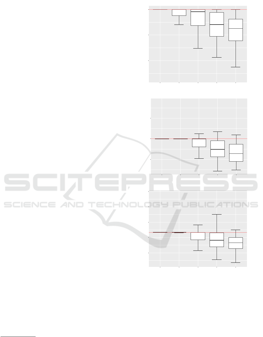
In order to make a fair comparison, we evaluate
the ratio of the proposed solution to the baseline so-
lution for each metric. Figure 3 shows a boxplot
3
for
each of the metrics. All three boxplots show that the
more activities are needed to perform during the day,
the bigger speed-up can be obtained from whole day
optimization. For five activities, which is still a very
reasonable number for an average user, the time spent
on a day activity plan may be more than 20% and
on average nearly 10% shorter using whole day opti-
mization. For an average 10h workday (including e.g.,
shopping), this accounts for 2 and 1 hour respectively
which is a very significant amount of time to be saved.
As already discussed, similar patterns can be ob-
served for the metrics for which the algorithm does not
explicitly optimize. Figure 3(b) shows that for five ac-
tivities a day, the proposed approach saves nearly 20%
energy (and subsequently charging costs) on average.
6.2 Effect of the Speed-Ups
In this section, we evaluate the effect of the pruning
speed-ups and the heuristic (Section 5) on the perfor-
mance of Algorithm 1 in terms of opened states, which
directly translates to the execution time. We decided
to use the opened states as the main performance mea-
3
The boxplots show median (strong line), mean (black
dot), the box showing Q1 (the 25th percentile) and Q3 (the
75th percentile) and the whiskers shows the lowest and high-
est point within 1.5 IQR of the lower and higher quartile
respectively. The outliers are shown as circles.
a)
●
●
●
●
●
●
●
●
●
●
●
●
●
●
●
●
●
●
●
●
●
●
●
●
●
●
0.8
0.9
1.0
1 2 3 4 5
Activities
Duration ratio
b)
●
●
●
●
●
●
●
●
●
●
●
●
●
●
●
●
●
●
●
●
●
●
●
●
●
●
●
●
●
●
●
●
●
●
●
●
●
●
●
●
●
●
●
●
●
●
●
●
●
●
●
●
●
●
●
●
●
●
●
●
●
●
●
●
●
●
●
●
●
●
●
●
●
●
●
●
●
●
0.75
1.00
1.25
1 2 3 4 5
Activities
Consumption ratio
c)
●
●
●
●
●
●
●
●
●
●
●
●
●
●
●
●
●
●
●
●
●
●
●
●
●
●
●
●
●
●
●
●
●
●
●
●
●
●
●
●
●
●
●
●
●
●
●
●
●
●
●
●
●
●
●
●
●
●
●
●
●
●
●
●
●
●
0.6
0.9
1.2
1.5
1.8
1 2 3 4 5
Activities
Cost ratio
Figure 3: Ratios of the single trip baseline and the proposed
whole day global approach in dependence on the number of
activities.
sure because it is independent of the experimentation
environment and immune to measurement errors (no
need to calculate the scenarios multiple times).
Figure 4 shows the comparison of ratios of the
opened states of the proposed solution without any
speed-ups and using the particular combination of
speed-ups. The combinations of speed-ups exclud-
ing the heuristic perform significantly worse than the
heuristic itself and any combination including it. The
Whole Day Mobility Planning with Electric Vehicles
161

●
●
●
●
●
●
●
●
●
●
●
●
●
●
●
●
●
●
●
●
●
●
●
●
●
●
●
●
●
●
●
●
●
●
●
●
●
●
●
●
●
●
●
●
●
●
●
●
●
●
●
●
●
●
●
●
●
●
●
●
●
●
●
●
●
●
●
●
●
●
●
●
●
●
●
●
●
●
●
●
●
●
●
●
●
●
●
0.00
0.25
0.50
0.75
1.00
[H]
[A]
[Ch]
[A,H]
[Ch,H]
[A,Ch]
[A,Ch,H]
Opened states
Figure 4: Opened states in dependence on the used speed-
ups relative to no speed-ups: H – heuristic (Section 5.3), A –
activity temporal consistency (Section 5.1), Ch – charging
consistency (Section 5.2).
best result is obtained by combining all speed-ups,
which is not surprising. The combination of all speed-
ups reduces the solution time by 90% on average,
which shows that the proposed speed-ups are a sig-
nificant improvement.
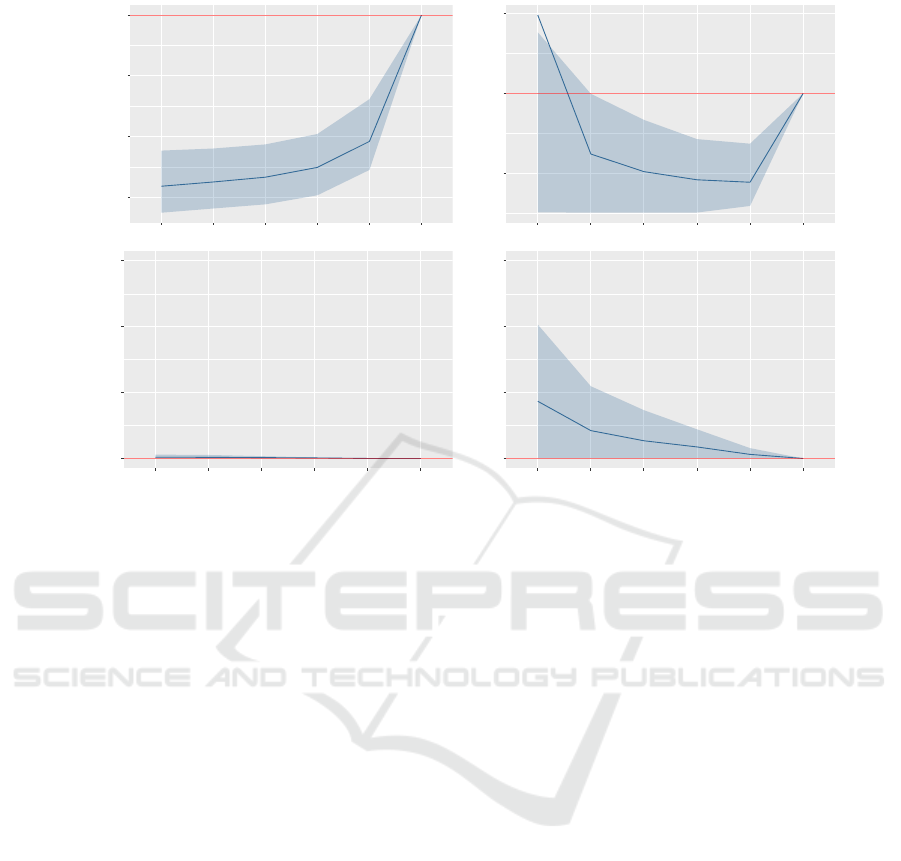
6.3 Effect of the Dominance Relaxation
The last set of experiments evaluates the performance
in terms of opened states and the quality of the so-
lution (the plan duration metric) when applying the
dominance relaxation speed-up. In this experiment
all speed-ups from the previous section (pruning and
heuristic) were used in combination with multiple set-
tings of dominance relaxation described in Section 5.4.
Figure 5 shows the ratios of the algorithm using
the given dominance relaxation value and using no
dominance relaxation. The left column shows the
SOC relaxation ε
β
which relaxes the dominance only
on the SOC, whereas the right column shows the cri-
teria relaxation ε
f
which relaxes the dominance on
the optimization function f (τ,γ) , which in our case
equals to the time τ . The results show that even though
the number of opened states are reduced to 50% with
SOC relaxation coefficient decreased from ε
β
= 1 to
ε
β
= 0.99 , the quality of the solution is practically
intact.
As expected, there is a significant decrease in the
number of states also with criteria relaxation coeffi-
cient set to ε
f
= 0.99 , but the impact on the plan dura-
tion is much greater than with SOC relaxation ε
β
. The
results suggest that the best trade-off between execu-
tion time and quality of the solution might be provided
by the combination of ε
β
= 0.99 and ε
f
= 0.99 . In-
deed, such a combination reduces the execution time
to 25% while not increasing the plan duration above
2.5% for 90% of the instances. An interesting result
is that lower criteria relaxation coefficient ε
f
leads to
a higher number of opened states. This is probably
caused by pruning away to many labels resulting in
exploration of number of detours which would not be
otherwise explored thanks to the heuristic.
7 CONCLUSION
In this work, we have proposed a novel Whole Day Mo-
bility Planning with Electric Vehicles (WDMEV) prob-
lem together with a label-setting algorithm to solve it.
We have shown that optimizing the WDMEV problem
significantly improves the results when compared to a
naive approach employed by humans in terms of plan
duration, energy efficiency and overall cost. Moreover,
we have provided a number of speed-ups and evaluated
their effect on performance of the algorithm.
ACKNOWLEDGEMENTS
This research was funded by the European Union
Horizon 2020 research and innovation programme un-
der the grant agreement N
◦
713864 and by the Grant
Agency of the Czech Technical University in Prague,
grant No. SGS16/235/OHK3/3T/13.
REFERENCES
Arslan, O., Yıldız, B., and Kara s¸ an, O. E. (2015). Min-
imum cost path problem for plug-in hybrid electric
vehicles. Transportation Research Part E: Logistics
and Transportation Review, 80:123 – 141.
Artmeier, A., Haselmayr, J., Leucker, M., and Sachenbacher,
M. (2010). The shortest path problem revisited: Opti-
mal routing for electric vehicles. In Annual Conference
on Artificial Intelligence, pages 309–316. Springer.
Bansal, N., Blum, A., Chawla, S., and Meyerson, A. (2004).
Approximation algorithms for deadline-tsp and vehi-
cle routing with time-windows. In Proceedings of the
thirty-sixth annual ACM symposium on Theory of com-
puting, pages 166–174. ACM.
Batista, L. S., Campelo, F., Guimar
˜
aes, F. G., and Ram
´
ırez,
J. A. (2011). A comparison of dominance criteria
in many-objective optimization problems. In Evolu-
tionary Computation (CEC), 2011 IEEE Congress on,
pages 2359–2366. IEEE.
Beasley, J. E. and Christofides, N. (1989). An algorithm for
the resource constrained shortest path problem. Net-
works, 19(4):379–394.
ICAART 2018 - 10th International Conference on Agents and Artificial Intelligence
162

SOC relaxation (ε
β
= x,ε
f
= 1) Criteria relaxation (ε
β
= 1, ε
f
= x)
Execution time ratio
●
●
●
●
●
●
0.25
0.50
0.75
1.00
0.9 0.93 0.95 0.97 0.99 1
●
●
●
●
●
●
0.5
1.0
1.5
0.9 0.93 0.95 0.97 0.99 1
Plan duration ratio
●
●
●
●
●
●
1.0
1.1
1.2
1.3
0.9 0.93 0.95 0.97 0.99 1
●
●
●
●
●
●
1.0
1.1
1.2
1.3
0.9 0.93 0.95 0.97 0.99 1
Figure 5: Effect of dominance relaxation on plan duration and execution time. The filled area represents data between the 1st
and the 9th quantile.
Desaulniers, G., Errico, F., Irnich, S., and Schneider, M.
(2016). Exact algorithms for electric vehicle-routing
problems with time windows. Operations Research,
64(6):1388–1405.
Desrochers, M. and Soumis, F. (1988). A generalized perma-
nent labelling algorithm for the shortest path problem
with time windows. INFOR: Information Systems and
Operational Research, 26(3):191–212.
Desrosiers, J., Dumas, Y., Solomon, M. M., and Soumis,
F. (1995). Time constrained routing and scheduling.
Handbooks in operations research and management
science, 8:35–139.
Dijkstra, E. W. (1959). A note on two problems in connexion
with graphs. Numerische mathematik, 1(1):269–271.
Dumas, Y., Desrosiers, J., Gelinas, E., and Solomon, M. M.
(1995). An optimal algorithm for the traveling sales-
man problem with time windows. Operations research,
43(2):367–371.
Eisner, J., Funke, S., and Storandt, S. (2011). Optimal route
planning for electric vehicles in large networks. In
AAAI, pages 1108–1113.
Felipe,
´
A., Ortu
˜
no, M. T., Righini, G., and Tirado, G. (2014).
A heuristic approach for the green vehicle routing prob-
lem with multiple technologies and partial recharges.
Transportation Research Part E: Logistics and Trans-
portation Review, 71:111–128.
Fi
ˇ
ser, T. (2017). Integrated route and charging planning for
electric vehicles. B.S. thesis, Czech Technical Univer-
sity in Prague.
Garey, M. R. and Johnson, D. S. (2002). Computers and
intractability, volume 29. wh freeman New York.
Hansen, P. (1980). Bicriterion path problems. In Multiple
criteria decision making theory and application, pages
109–127. Springer.
Hart, P. E., Nilsson, N. J., and Raphael, B. (1968). A for-
mal basis for the heuristic determination of minimum
cost paths. IEEE transactions on Systems Science and
Cybernetics, 4(2):100–107.
Ioachim, I., Gelinas, S., Soumis, F., and Desrosiers, J. (1998).
A dynamic programming algorithm for the shortest
path problem with time windows and linear node costs.
Networks, 31(3):193–204.
Khuller, S., Malekian, A., and Mestre, J. (2011). To fill or
not to fill: The gas station problem. ACM Transactions
on Algorithms (TALG), 7(3):36.
Krentel, M. W. (1988). The complexity of optimization
problems. Journal of computer and system sciences,
36(3):490–509.
Li, F., Cheng, D., Hadjieleftheriou, M., Kollios, G., and
Teng, S.-H. (2005). On trip planning queries in spatial
databases. In International Symposium on Spatial and
Temporal Databases, pages 273–290. Springer.
Ma, X., Shekhar, S., and Xiong, H. (2009). Multi-type
nearest neighbor queries in road networks with time
window constraints. In Proceedings of the 17th ACM
SIGSPATIAL International Conference on Advances
in Geographic Information Systems, GIS ’09, pages
484–487, New York, NY, USA. ACM.
Nemhauser, G. L. (1972). A generalized permanent label
setting algorithm for the shortest path between spec-
ified nodes. Journal of Mathematical Analysis and
Applications, 38(2):328–334.
Whole Day Mobility Planning with Electric Vehicles
163

Rice, M. N. and Tsotras, V. J. (2013). Parameterized al-
gorithms for generalized traveling salesman problems
in road networks. In Proceedings of the 21st ACM
SIGSPATIAL International Conference on Advances
in Geographic Information Systems, SIGSPATIAL’13,
pages 114–123, New York, NY, USA. ACM.
Sachenbacher, M., Leucker, M., Artmeier, A., and Hasel-
mayr, J. (2011). Efficient energy-optimal routing for
electric vehicles. In AAAI.
Schneider, M., Stenger, A., and Goeke, D. (2014). The elec-
tric vehicle-routing problem with time windows and
recharging stations. Transportation Science, 48(4):500–
520.
Veneti, A., Konstantopoulos, C., and Pantziou, G. (2016).
Time-dependent bi-objective itinerary planning algo-
rithm: Application in sea transportation. In OASIcs-
OpenAccess Series in Informatics, volume 54. Schloss
Dagstuhl-Leibniz-Zentrum fuer Informatik.
ICAART 2018 - 10th International Conference on Agents and Artificial Intelligence
164