Real-time Low SNR Signal Processing for Nanoparticle Analysis with

Deep Neural Networks

Jan Eric Lenssen

, Anas Toma

, Albert Seebold

, Victoria Shpacovitch

, Pascal Libuschewski

Frank Weichert

, Jian-Jia Chen

and Roland Hergenr

oder

CS VII - Computer Graphics, TU Dortmund University, Otto-Hahn-Straße 16, 44227 Dortmund, Germany

CS XII - Embedded Systems, TU Dortmund University, Otto-Hahn-Straße 16, 44227 Dortmund, Germany

Leibniz-Institute for Analytical Science, ISAS e.V., Bunsen-Kirchhoff-Straße 11, 44139 Dortmund, Germany

Keywords:

Nanoparticle Analysis, Deep Learning, Convolutional Neural Network, GPGPU Real Time Processing,

Biosensing.

Abstract:

In this work, we improve several steps of our PLASMON ASSISTED MICROSCOPY OF NANO-SIZED OBJECTS

(PAMONO) sensor data processing pipeline through application of deep neural networks. The PAMONO-

biosensor is a mobile nanoparticle sensor utilizing SURFACE PLASMON RESONANCE (SPR) imaging for

quantiﬁcation and analysis of nanoparticles in liquid or air samples. Characteristics of PAMONO sensor

data are spatiotemporal blob-like structures with very low SIGNAL-TO-NOISE RATIO (SNR), which indicate

particle bindings and can be automatically analyzed with image processing methods. We propose and evaluate

deep neural network architectures for spatiotemporal detection, time-series analysis and classiﬁcation. We

compare them to traditional methods like frequency domain or polygon shape features classiﬁed by a Random

Forest classiﬁer. It is shown that the application of deep learning enables our data processing pipeline to

automatically detect and quantify 80 nm polystyrene particles and pushes the limits in blob detection with very

low SNRs below one. In addition, we present benchmarks and show that real-time processing is achievable on

consumer level desktop GRAPHICS PROCESSING UNITs (GPUs).

1 INTRODUCTION

The effect of SURFACE PLASMON RESONANCE

(SPR) is often utilized to study interactions between

different types of biomolecules (nucleic acids, pep-

tides, lipids, proteins, etc.) and to determine con-

centrations and afﬁnity constants of biomolecules in

solutions. The high sensitivity of SPR has led to a

common use of SPR sensors for real-time measure-

ments of biomolecule binding efﬁciency. However,

the task to quantify individual biological nanoparti-

cles with SPR sensors remained unsolved for a long

time.

Recently, the PLASMON ASSISTED MI-

CROSCOPY OF NANO-SIZED OBJECTS (PAMONO)

sensor was shown to overcome the limitation of

SPR to quantify individual biological nanoparticles

(Zybin, 2010; Zybin, 2013; Shpacovitch et al.,

2015): single viruses, virus-like particles and other

nanoparticles can be detected in suspensions of liquid

or air.

Manually analyzing the sensor data and quantify

the particles is a time-consuming task. An evalua-

tion of a single data set by an expert with a few hun-

dred particles can take several hours. The application

of a highly optimized GENERAL-PURPOSE COMPUT-

ING ON GRAPHICS PROCESSING UNITS (GPGPU)

pipeline (Siedhoff, 2016; Libuschewski, 2017) makes

it possible to automatically analyze the sensor data

and quantifying the nanoparticles in less than three

minutes. This enables the real-time measurements

of SPR sensors also for the PAMONO sensor. For

this automatic analysis, it was shown that it can re-

liably detect signals with an SNR down to 1.2 and

therefore, virus-like and polystyrene particles down

to 100 nm in our experiment setup (Siedhoff, 2016;

Libuschewski, 2017; Siedhoff et al., 2014). Automat-

ically detecting SPR signals with lower SNR has yet

to be accomplished.

In this work, we push the limits of our meth-

ods and move towards the goal of detecting particle

signals with an SNR below one in PAMONO sen-

sor data by incorporating three different deep neural

networks for nanoparticle analysis into our GPGPU

Lenssen, J., Toma, A., Seebold, A., Shpacovitch, V., Libuschewski, P., Weichert, F., Chen, J-J. and Hergenröder, R.

Real-time Low SNR Signal Processing for Nanoparticle Analysis with Deep Neural Networks.

DOI: 10.5220/0006596400360047

In Proceedings of the 11th International Joint Conference on Biomedical Engineering Systems and Technologies (BIOSTEC 2018) - Volume 4: BIOSIGNALS, pages 36-47

ISBN: 978-989-758-279-0

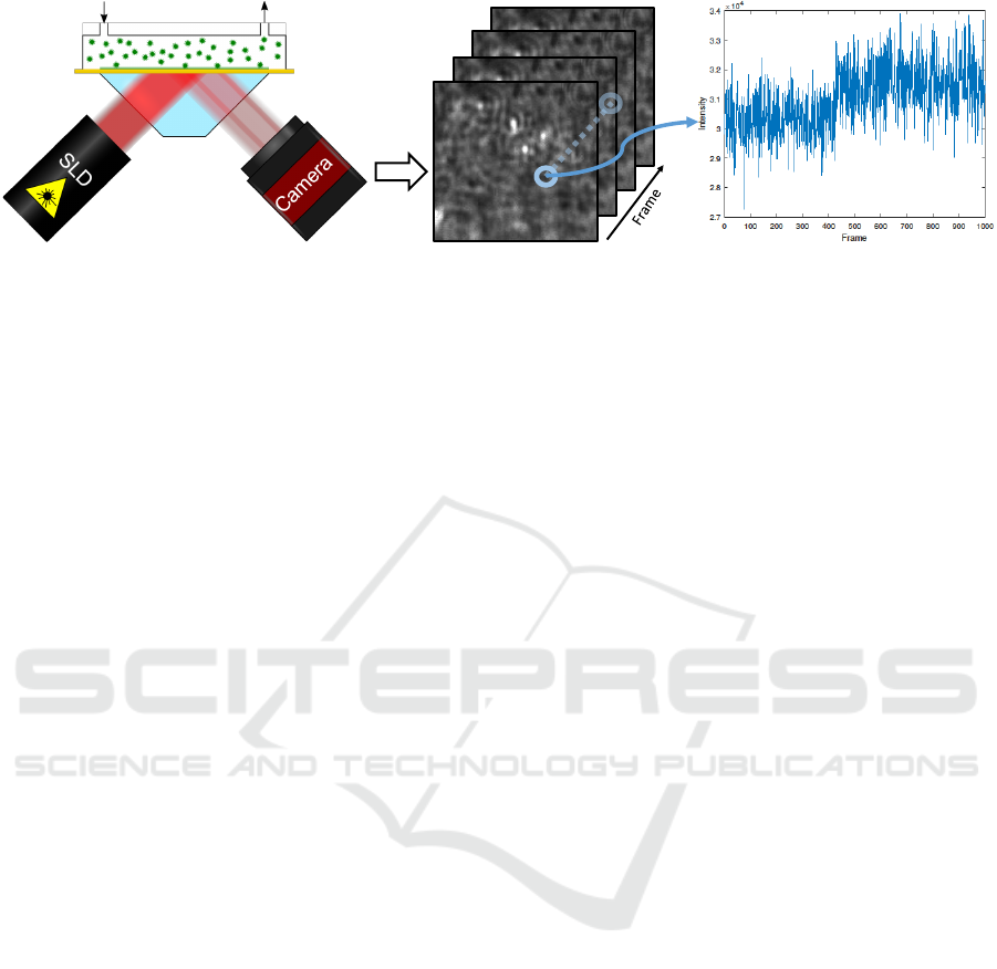
Figure 1: Principle of operation of the PAMONO sensor. It consists of a laser, the ﬂow cell, gold plate, and prism, and the

camera, as it is shown in the scheme. Nanoparticles attached to the gold layer result in refractive index changes of the surface,

which can be observed by the camera. On the captured image sequences, temporal intensity steps appear on particle binding

spots. Figure adapted from (Libuschewski, 2017).

pipeline: a spatiotemporal FULLY CONVOLUTIONAL

NETWORK (FCN) (Long et al., 2015), a time-series

analysis network (both for detection) and a CON-

VOLUTIONAL NEURAL NETWORK (CNN) (LeCun

et al., 1995) for classiﬁcation. In our experimental

setup, this enables the quantiﬁcation of 80 nm parti-

cles.

We evaluate those methods by performing two dif-

ferent types of experiments: a standalone classiﬁca-

tion evaluation where we test and compare classiﬁca-

tion methods on a dedicated benchmark data set and

a sensor data experiment where we apply our whole

processing pipeline on real sensor data. We show that

the proposed methods are able to achieve reliable re-

sults for sensor data containing particle signals with

an SIGNAL-TO-NOISE RATIO (SNR) below one, and

that the pipeline still fulﬁlls the soft real-time property

on current GRAPHICS PROCESSING UNITs (GPUs),

which means that on average, the data is processed

with at least the same speed as the sensor provides it.

2 PAMONO-Biosensor

The PAMONO sensor utilizes a Kretschmann’s

scheme (Kretschmann, 1971) of plasmon excitation to

detect individual particles. In Kretschmann’s conﬁg-

uration, as shown in Figure 1, an incident laser beam

passes through a glass prism, which is coated with

a very thin gold ﬁlm on one side. This ﬁlm forms

a sensor surface, on which the interactions between

biomolecules occur. At a certain angle of incidence

(resonance angle), an incidence beam is not reﬂected

and the gold sensor surface is very sensitive to any

changes of the refractive index near it. Any changes

of the refractive index in close vicinity of the gold

interface result in changes of reﬂection conditions.

Thus, any binding of a particle to the gold surface re-

stores the local reﬂection on the binding spot.

The data characteristic of particle signals in cap-

tured images, as shown in Figure 1, is as follows: On

places with plasmon excitation through particle bind-

ings, an increase of intensity in the time dimension

(intensity step) can be observed in the corresponding

pixels. In the spatial dimensions, these pixels form

a blob with surrounding wave-like structures. Both

variations in intensity are indications for a particle

binding and can be detected and analyzed by image

processing methods.

3 RELATED WORK

In the following we provide a broad context for

nanoparticle analysis in Section 3.1, before we out-

line the related work for our data processing methods.

Analyzing PAMONO sensor data is most related to

the ﬁeld of low SNR blob detection. Therefore, we

give a short overview about this subject in Section 3.2.

3.1 Nanoparticle Detection

When comparing SPR-based approaches to study bio-

logical nanoparticles, one should highlight the follow-

ing differences. Conventional SPR sensors deal with

the formation of a layer of biomolecules or biopar-

ticles onto a gold sensor surface and harnesses the

integral changes of reﬂectivity conditions to char-

acterize the layer assembly process. In contrast,

the PAMONO sensor utilizes local changes of re-

ﬂectivity to show individual biological nanoparti-

cles. Firstly, the latter issue makes the PAMONO

sensor more sensitive in the detection and quan-

tiﬁcation of biological nanoparticles. Secondary,

the PAMONO sensor provides direct information

about particle binding events. This helps to ob-

viate complex calculations of particle concentra-

tions based on the thickness of the particle layer

Real-time Low SNR Signal Processing for Nanoparticle Analysis with Deep Neural Networks

formed onto the sensor surface. Examples of other

nanoparticle analysis methods are SURFACE PLAS-

MON RESONANCE IMAGING (SPRi) (Steiner and

Salzer, 2001), NANOPARTICLE TRACKING ANALY-

SIS (NTA) (Dragovic et al., 2011), plaque assay (Dul-

becco, 1954), and ENZYME-LINKED IMMUNO-SOR-

BENT ASSAY (ELISA) (Gan and Patel, 2013). A

comprehensive overview about the plasmon reso-

nance effect is given by Pattnaik (Pattnaik, 2005).

Most similar to the PAMONO sensor are SPRi

sensors which are a wide spread technology that are

applied in a large ﬁeld of applications (Beusink et al.,

2008; Chinowsky et al., 2004; Giebel et al., 1999;

Naimushin et al., 2003; Scarano et al., 2011). Steiner

et al. states that the reason for the advantage of SPRi-

based methods is that they show speciﬁc bounds of

unlabeled molecules under in-situ conditions (Steiner

and Salzer, 2001), which also holds for the PAMONO

sensor.

3.2 Low SNR Blob Detection

Low SNR blob detection is the most related task to

our PAMONO data analysis, as small blob-like struc-

tures need to be identiﬁed in gray-scale images. Most

methods that are comparable to our pipeline can han-

dle an SNR down to four (Cheezum et al., 2001) or

two (Smal et al., 2009)

Automatic tumor detection in breast ultrasound

images represents a similar task to PAMONO image

processing. Moon et al. (Moon et al., 2013) compute

features by convolving partial derivatives of a Gaus-

sian distribution with the input images to solve this

task and Liu et al. (Liu et al., 2010) apply this method

to detect blobs in natural scenes.

Another related task is ﬁnding blobs in images

from ﬂuorescence microscopy, which was surveyed

by Cheezum et al. (Cheezum et al., 2001). It should

be noted that for the analyzed tracking tasks, an SNR

of four was required for the surveyed algorithms to

succeed. For PAMONO signals however, SNRs be-

low one need to be handled.

For live-cell ﬂuorescence microscopy, different

spot detection methods have been surveyed by Smal

et al. (Smal et al., 2009). It is stated that most classical

methods need an SNR of four to work. After present-

ing algorithms for SNRs down to two, they recom-

mend using supervised machine learning methods for

data with low SNR. The deep neural networks used in

this work fall under this category.

4 METHODS FOR AUTOMATED

NANOPARTICLE DETECTION

The following section details our methods for

nanoparticle analysis. First, an overview about the

data processing pipeline is given in Section 4.1. In

Section 4.2 we describe our deep neural network

models for detection and classiﬁcation and in Sec-

tion 4.3 we outline our frequency domain methods for

comparison. Last, implementation details are given in

Section 4.4.

4.1 Image Processing Pipeline -

overview

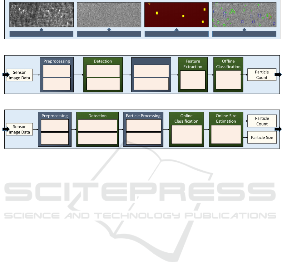
An overview of the image processing pipeline is given

in Figure 2. Figure 2a shows the overall detection task

with example images: First, a raw image. Second,

an image with removed background. Third, detected

particle pixels as binary heat map. Finally, generated

particle candidates.

Figure 2b shows the existing PAMONO sensor

data processing pipeline from previous work (Sied-

hoff, 2016; Libuschewski, 2017), which makes use

of several traditional image processing methods. It

consists of the steps preprocessing, detection, particle

processing, feature extraction and ofﬂine classiﬁca-

tion. The input is a sequence of sensor images and

the output is the particle count and the spatiotempo-

ral coordinates of each particle. The detection step

estimates a binary heat map marking possible par-

ticle signal positions. After the detection step, the

heat map is further processed to generate polygon

proposals. These polygons are matched over time to

obtain particle candidates that are visible over sev-

eral frames. Subsequently, polygon features are ex-

tracted and the particle candidates are either classiﬁed

as true particle or artifact/noise in an ofﬂine step, us-

ing a Random Forest classiﬁer (Breiman, 2001). This

pipeline consists of a large number of image process-

ing methods that can be chosen and conﬁgured by pa-

rameter sets (Libuschewski, 2017). In addition, Sied-

hoff developed the SynOpSis approach to automati-

cally optimize parameter sets towards speciﬁc tasks,

using synthetic sensor data (Siedhoff, 2016).

Figure 2c shows our proposed processing pipeline,

which incorporates novel methods from the ﬁeld of

deep learning: a FULLY CONVOLUTIONAL NET-

WORK (FCN) and a time-series analysis replace the

detection step, a CONVOLUTIONAL NEURAL NET-

WORK (CNN) online classiﬁcation replaces the fea-

ture extraction and classiﬁcation step and an addi-

tional CNN for online size estimation is added. The

online particle size estimation network is able to de-

BIOSIGNALS 2018 - 11th International Conference on Bio-inspired Systems and Signal Processing

Detected Particle Pixels

Background Removed

Raw Data

Particle Candidates

(a) Detection task overview.

Background

Elimination

Template

Matching

Particle Processing

Candidate

Generation

Patch Extraction

Random

Forrest

Classifier

Noise

Reduction

Time-Series

Analysis

Polygon

Shape

Features

(b) Baseline processing pipeline from previous work.

Background

Elimination

Fully Convolutional

Network

Candidate

Generation

Patch Extraction

Convolutional

Neural

Network

Noise

Reduction

Convolutional

Neural

Network

Time-Series

Analysis Network

Figure 2: An overview of the detection task, the baseline processing pipeline and the proposed processing pipeline. Traditional

image processing methods have been replaced by deep neural networks.

rive the size of individual particles, which is part of

previous work (Lenssen et al., 2017) but mentioned

here for the sake of completeness. All networks are

detailed in the following section.

Both pipelines follow the signal model

I(x, y,t) = B(x, y) · (T · A)(x, y,t) +N(x, y,t) (1)

where I is the sensor image sequence, T ·A represents

particle and artifact signals and N is additive noise

(Siedhoff, 2016). Given the sensor image sequence

I, we can approximate the particle and artifact signal

T · A by removing the constant-over-time background

signal B. This is done by dividing the current image in

the sequence by the mean of a set of previous frames.

Thus, only the non-constant parts, particle signals, ar-

tifacts and noise remains in the images. Then, the de-

tection and classiﬁcation steps aim to distinguish the

particle signal P from artifact A and noise N. In the

following sections we provide details of our proposed

methods.

4.2 Deep Neural Networks

We present three different neural network architec-

tures for marking pixels that belong to a particle (de-

tection) and to sort out false detections (classiﬁca-

tion). For the detection task, we present two different

approaches which we evaluate against each other. All

networks are trained using the cross entropy loss

L = −

∑

i=1

· log

, (2)

where

is the softmax output of the network and y

is a binary one-hot vector indicating the correct class.

For the detection FCN, we compute the pixel-wise

loss and average over the N pixels of all images in

one mini-batch while for the remaining networks, the

cross entropy is only averaged over all N examples in

one mini-batch.

While choosing the neural network architectures,

we were driven by two different goals: high accuracy

and low inference execution time to maintain the soft

real-time property. To achieve the second goal we

heavily make use of the two following concepts:

• Convolutional layers with 1 × 1 ﬁlters: Strictly

speaking, those layers do not perform a con-

volution but combine the features of each pixel

densely to a new set of features while sharing the

trained weights over all pixels. In a CNN, some

classical convolutional layers can be replaced by

those layers to save execution time without losing

much accuracy.

• Feature reduction layers: As ﬁrst applied in

the Inception Modules of the GoogleNet (Szegedy

et al., 2015), 1 × 1 convolution layers can be used

to reduce the number of features on each pixel be-

fore applying the next layer, which also has shown

Real-time Low SNR Signal Processing for Nanoparticle Analysis with Deep Neural Networks

Input Image Sequence - 8

2-Class Confidence Map

Conv. Layer 3x3 - 32

Max-Pooling - 32

Max-Pooling - 64

Conv. Layer 1x1 - 2

Upscaling x4

Fire Module – 8 / 64

Conv. 1x1 – Feature Reduce - 8

Conv. 3x3 - 32

Conv. 1x1 - 32

Filter Concatenation - 64

Fire Module – 8 / 64

Conv. 1x1 – Feature Reduce - 8

Conv. 3x3 - 32 Conv. 1x1 - 32

Filter Concatenation - 64

(a) Fully conv. detection network.

Conv. Layer 1x1 – 80

(Pixel-wise Fully-Connected)

Input Image Sequence - 32

Conv. Layer 1x1 - 64

(Pixel-wise Fully-Connected)

Conv. Layer 1x1 – 48

(Pixel-wise Fully-Connected)

Conv. Layer 1x1 – 32

(Pixel-wise Fully-Connected)

Conv. Layer 1x1 – 2

(Pixel-wise Fully-Connected)

2-Class Confidence Map

(b) Time-series analysis network.

Input Image Patch

2- Class Softmax Output

Conv. Layer 3x3 - 64

Max-Pooling - 64

Max-Pooling - 128

Conv. Layer 1x1 - 64

Fire Module – 16 / 128

Max-Pooling - 128

Fire Module – 16 / 128

Max-Pooling - 128

Fire Module – 16 / 128

Average-Pooling - 64

Fully-Connected - 2

Figure 3: Architectures of our two different detection and our classiﬁcation network. After the layer description, the number

of output feature maps is given for each layer. In each ﬁgure, the input is shown on the bottom and the output on the top.

to save execution time without sacriﬁcing much

accuracy.

Fully-Convolutional Detection Network. The

ﬁrst detection network combines the ideas of the

FCNs from Long et al. (Long et al., 2015) with the

efﬁciency of the inception modules of the GoogleNet

(Szegedy et al., 2015) and the spatial-temporal

early fusion method mentioned by Karpathy et al.

(Karpathy et al., 2014). The architecture is shown

in Figure 3a. As network input, we use a stack of 8

subsequent input images from the sensor data stream.

Then, the images are processed using scaled-down

inception modules, called ﬁre modules, and max

pooling. The ﬁre modules, as employed in the

SqueezeNet (Iandola et al., 2016), consist of three

convolutional layers. First the data is reduced by

applying a 1 ×1 convolutional layer. Then, the num-

ber of features is expanded again by another 1 ×1

and one 3 × 3 convolutional layer before both results

are concatenated along the feature dimension. After

three ﬁre modules and max pooling layers, the down-

scaled feature maps are upscaled to input resolution

before computing the pixel-wise loss. As training

data, we use stacks of real sensor images together

with binary ground truth images that were automat-

ically derived from the manually created ground truth.

Time-Series Analysis Network. The second detec-

tion approach classiﬁes the signal in a single pixel

over time. This has been accomplished with a 2-class,

5-layer MULTILAYER PERCEPTRON (MLP) classi-

ﬁer. The input time-series consists of 32 signal values,

normalized to zero mean and a standard deviation of

one. Although this classiﬁcation network is based on

an MLP architecture, it was realized using convolu-

tional layers, due to performance and practical rea-

sons on this particular application. The MLP classi-

ﬁer realized as CNN is shown in Figure 3b. Since

the detection runs on an image sequence, the three-

dimensional inputs can be used as input for a CNN

with 1 ×1 convolutional layers, which yields a two-

dimensional feature map with the same width and

height as a single input image. Hence, every layer

in this CNN consists of n 1 × 1 ﬁlters, which is equiv-

alent to the densely connected layer with n outputs of

the MLP, applied on each pixel, individually.

The time-series classiﬁcation network was trained

exclusively on synthesized data, which is motivated

by the fact that it is easier and more accurate to

generate realistic pixel time-series than it is to

manually label real data. The training data set

is composed of 5000 000 positive and 5000 000

negative training samples. The negative samples

consist of values drawn from a Gaussian distribution

N (µ, σ

), where means 0.1 ≤ µ ≤ 0.9 and standard

deviations 0.005 ≤ σ ≤ 0.25 are uniformly sampled

for each sample. For the positive examples, the same

procedure was used and an intensity step with step

height depending on target particle size was added on

top.

Particle Classiﬁcation Network. We decided to

employ an independent classiﬁcation CNN (LeCun

et al., 1995) after candidate generation to classify

between correct detections (particles) and false

detections (artifacts and noise). Since this network

BIOSIGNALS 2018 - 11th International Conference on Bio-inspired Systems and Signal Processing

is only applied on small signal patches, it allows the

application of a deeper network and more ﬁlters per

layer without destroying the real-time property. Our

classiﬁcation architecture is displayed in Figure 3c.

It also makes use of SqueezeNet’s FireModules since

they have proven to be very fast and effective. As

input, the network receives 32 px × 32 px patches

while the output are conﬁdences for two classes. The

network is trained using a set of signals that was

extracted from real sensor data, as described further

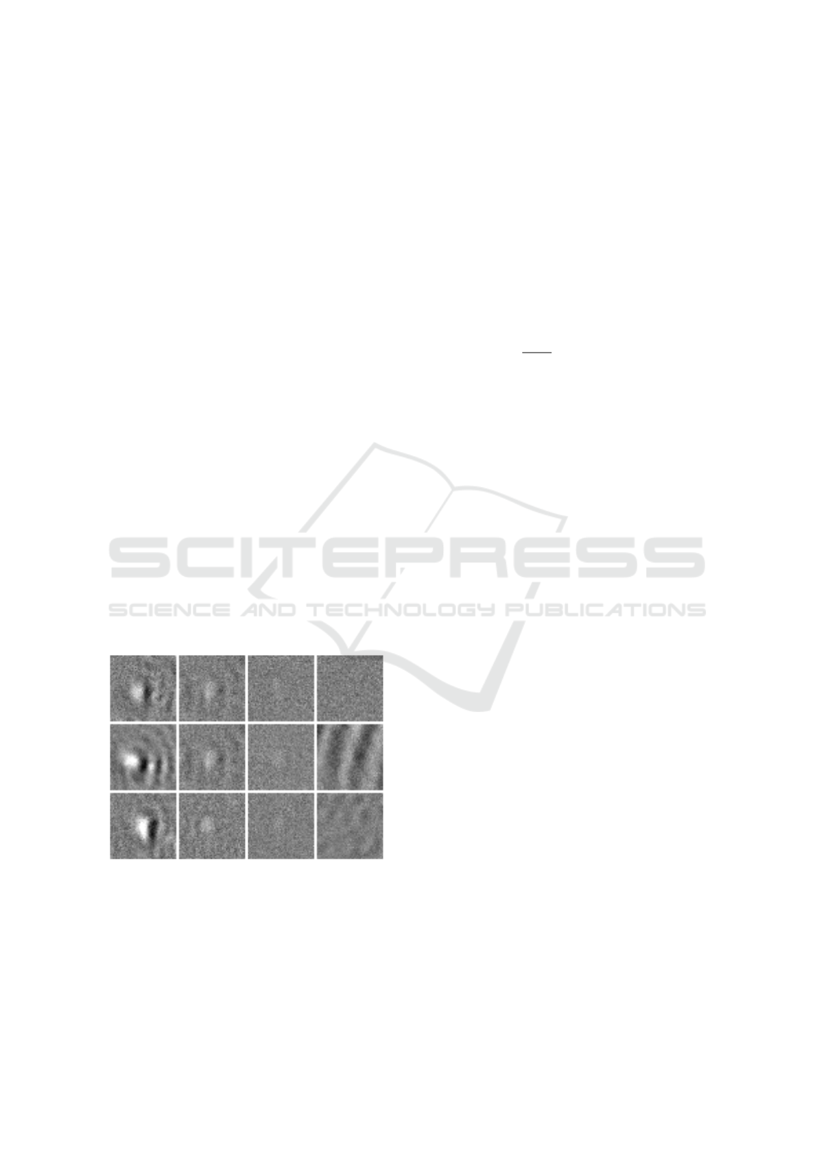
in Section 5 and shown in Figure 4.

Particle Size Estimation Network. The particle size

estimation is part of the previous work (Lenssen et al.,

2017) and is mentioned here for the sake of com-

pleteness. It consists of a CNN that simulates regres-

sion with classiﬁcation through binning of the particle

sizes. It is trained using synthesized particle patches

containing averaged intensity peaks.

4.3 Frequency Domain Analysis

Frequency domain analysis has been used in the lit-

erature to detect the abnormalities in medical im-

ages (Aljarrah et al., 2015; Woodward et al., 2003).

We use it to compare our classiﬁcation network to

a traditional approach on the same task. We extract

two types of frequency domain features, spectral and

wavelets features, to analyze the texture of the im-

age, because images that contain particles have dif-

ferent texture than images without particles, as shown

in Figure 4.

Figure 4: Example patches extracted from the sensor data.

The ﬁrst three columns show signals of 200 nm, 100 nm and

80 nm particles, respectively. The fourth column displays

patches containing only noise and artifact signals without

particles. The images have been manually enhanced for vi-

sualization.

Spectral features can be used to characterize the

periodicity of the texture pattern by observing the

bursts in Fourier spectrum of the image. The features

include the peak value and its location, the mean, the

variance, and the distance between the mean and the

peak value of the spectrum (Gonzalez and Woods,

2006). Wavelet transform analysis is also used to de-

tect the particles by studying the frequency content of

the image in different scales. We use the Haar wavelet

transform with 3 scales to produce the coefﬁcients for

10 channels. The energy values of the channels rep-

resent the texture features, which can be extracted by

calculating the mean magnitude of each channel’s co-

efﬁcients as follows:

E =

M · N

∑

i=1

∑

j=1

| w(i, j) |, (3)

where M and N are the dimensions of the channel,

and w(i, j) is the wavelet coefﬁcient (Castellano et al.,

2004). To classify the patches based on the extracted

features a Random Forest classiﬁer was used.

4.4 Implementation Details

The following section presents details and parameters

of the training of neural networks, the Random Forest

classiﬁers and the pipeline implementations we used

to obtain our results.

Neural Network Training. The FCN and CNNs

were trained with TensorFlow (Abadi et al., 2015)

using the backpropagation algorithm (Hecht-Nielsen

et al., 1988) for gradient estimation and the Adam

optimization method (Kingma and Ba, 2014) with

an initial step size α = 0.001, exponential decay

rates β

= 0.9 and β

= 0.999, and ε = 10

−8

. In

contrast, the time-series analysis network was trained

with the ADAGRAD optimization method (Duchi

et al., 2011) with an initial step of α = 0.01 and an

exponential decay rate of 0.9. As mini-batch sizes,

we used 16 for the FCN detector and 256 for the

classiﬁcation networks. The parameter settings were

chosen empirically based on preliminary work.

Training Data Augmentation. In addition to

dropout, we applied different data augmentation

techniques to further reduce overﬁtting. For the

input of the FCN detector and the CNN classiﬁer

we applied small random intensity and contrast

modiﬁcations as well as random ﬂipping. Intensity

and contrast modiﬁcations are always applied on the

whole image so that relative intensity information is

preserved. In addition to that, the 32 px × 32 px input

patches for classiﬁcation are randomly cropped out

of 48 px × 48 px images. It should be noted that the

intensity input of the size estimation network is not

Real-time Low SNR Signal Processing for Nanoparticle Analysis with Deep Neural Networks

Table 1: Generated patches and captured image sequences used for evaluation with average particle size, number of

patches/frames, number of particles and median SNR.

Particle classiﬁcation data sets Avg. part. size # Training images # Testing images

Ds1

Patches

100&200nm

100 nm & 200 nm 19344 19344

Ds2

Patches

80nm

80 nm 8308 8308

Ds3

Patches

80nm

80 nm 12916 3700

Sensor experiment data sets Avg. part. size # Frames # Part. Median SNR

Ds4

200nm

200 nm 2000 93 2.125

Ds5

100nm

100 nm 4000 56 1.247

Ds6

80nm

80 nm 6300 819 0.761

Ds7

80nm

80 nm 6750 214 0.716

Ds8

80nm

80 nm 4400 196 0.639

modiﬁed, since the absolute intensity holds important

information about particle size.

Random Forest Classiﬁer. The Random Forest

classiﬁer model has been trained with Weka (Hall

et al., 2009). A cross validation parameter tun-

ing (Kohavi, 1995) has been performed to optimize

the hyper-parameters of the Random Forest model.

The maximum depth of the trees has been optimized

from 5 to 20, the number of trees from 100 to 500,

and the number of random features from 4 to 9.

Image Processing Pipeline. The GPGPU image pro-

cessing pipeline, called VIRUS DETECTION WITH

OPENCL (VirusDetectionCL), was described and im-

plemented by Libuschewski using OPEN COMPUT-

ING LANGUAGE (OpenCL) (Libuschewski, 2017).

For real-time neural network inference, we use

DEEP RESOURCE-AWARE OPENCL INFERENCE

NETWORKS (deepRacin), an OpenCL-based neural

network inference library we created. Using this li-

brary, we are able to directly integrate our trained

networks into the VirusDetectionCL pipeline and ex-

ecute them on OpenCL-capable mobile and desktop

devices, utilizing the parallel processing power of

GPUs.

5 EXPERIMENTS

We provide results for two different types of experi-

ments. First, we solely evaluate the classiﬁcation net-

work using dedicated classiﬁcation benchmark data

sets, for which examples were given in Figure 4. Sub-

sequently, we use the whole pipeline, including de-

tection and classiﬁcation networks, to analyze sensor

data.

The main focus is on the 80 nm data sets, which

have very low SNR. The SNR(S, B) for a given par-

ticle signal S and a given background signal B is cal-

culated according to the deﬁnition of Cheezum et al.

(Cheezum et al., 2001) as

SNR(S, B) =

|µ(S) − µ(B)|

σ(S)

, (4)

where S is a multiset of signal values, B a multiset

of background values, µ(S) the average of S, µ(B) the

average of B and σ(S) the standard deviation of S.

5.1 Data Set Acquisition

For capturing nanoparticles with the PAMONO sen-

sor we used glass slides covered with a layer of about

50 nm thickness encompassing 5 nm Titanium and ap-

proximately 45 nm gold (PHASIS, Switzerland) for

the sensor surface. A liquid containing around 10 %

of aluminum hydroxide (N

uscoﬂock, Dr. N

usgen

Chemie, Germany) was employed to cover the gold

layer. These gold bearing glass slides were attached

to the glass prism with a help of an immersion liq-

uid possessing the same refractive index as the prism.

A diode laser (HL6750MG, Thorlabs, Germany) pro-

vided an incidence beam with a wavelength λ ≈

675 nm for illumination of the gold layer through the

prism. A 50 mm photographic lens (Rokkor MD, Mi-

nolta, Japan) imaged the gold surface onto a 5 Mpx

camera (GC2450 Prosilica, Allied Vision, Germany).

Polystyrene nanoparticles (Molecular Probes, Life

Technologies, USA) of 200 nm, 100 nm and 80 nm

were pumped through the U-shaped ﬂow cell as a

suspension in distilled water containing 0.3 % sodium

chloride. Image recording speed was 41 fps to 45 fps,

but was kept constant during each experiment. For

each suspension of 80 nm, 100 nm and 200 nm par-

ticles, image sequences were captured, picturing the

sensor surface.

BIOSIGNALS 2018 - 11th International Conference on Bio-inspired Systems and Signal Processing

The resulting data sets are listed in Table 1. The

ﬁrst three data sets, named Ds1

Patches

100&200nm

, Ds2

Patches

80nm

and Ds3

Patches

80nm

contain extracted patches from the

recorded signal, cf. Figure 4, and the subsequent

ﬁve data sets, named Ds4

200nm

, Ds5

100nm

, Ds6

80nm

Ds7

80nm

and Ds8

80nm

are raw sensor image sequences

as recorded by the sensor. For all data sets, manually

created ground truths are available in which all parti-

cle signals were marked by human annotators.

5.2 Standalone Classiﬁcation

Experiment

The ﬁrst three data sets in Table 1 are benchmark

data sets for particle classiﬁcation. They are used

to evaluate the classiﬁcation CNN and the frequency

domain analysis and consist of 48 px × 48 px particle

signal patches, which were extracted from sensor sig-

nal. Data set Ds1

Patches

100&200nm

contains disjoint training

and testing patches extracted from data sets Ds4

200nm

and Ds5

100nm

. Data sets Ds2

Patches

80nm

and Ds3

Patches

80nm

contain patches from data sets Ds6

80nm

and Ds7

80nm

For data set Ds2

Patches

80nm

training and testing images are

drawn from both source data sets while for Ds3

Patches

80nm

training images are only extracted from Ds6

80nm

and

testing images from Ds7

80nm

, thus allowing to evalu-

ate the transferability of the model between different

measurements. In all 3 generated data sets, training

and testing data are disjoint and class-balanced, al-

lowing to use accuracy as quality measure.

We applied two different methods on these data

sets: the CNN classiﬁer called M

CNN-Cl

and the fre-

quency domain analysis with Random Forest classi-

ﬁer called M

FDA

5.3 Sensor Data Experiment

We evaluate the whole processing pipeline by com-

paring the results (proposed particles that were posi-

tively classiﬁed) to the manually created ground truth.

Data set Ds6

80nm

was used for training the detector

and classiﬁcation network. The trained models were

tested on data sets Ds4

200nm

, Ds5

100nm

, Ds7

80nm

and

Ds8

80nm

As quality measures, precision, recall and the F

score (Powers, 2011) are used. The F

-score is de-

ﬁned as a balance between precision and recall:

2 · precision · recall

precision + recall

. (5)

We differentiate between results obtained by apply-

ing the detection step only and that obtained by de-

tecting and classifying. Ideally, the detector provides

high recall while the classiﬁcation is able to sort out

false positives without sorting out too many true pos-

itives. Therefore, we applied and compared ﬁve dif-

ferent methods:

• M

Baseline

: baseline pipeline (previous work),

• M1

FCN-Det

: the FCN detector without classiﬁca-

tion,

• M2

FCN-Det

CNN-Cl

: the FCN detector with CNN classiﬁ-

cation,

• M3

TS-Det

: the time-series analysis network with-

out classiﬁcation,

• M4

TS-Det

CNN-Cl

: the time-series detection network with

CNN classiﬁcation.

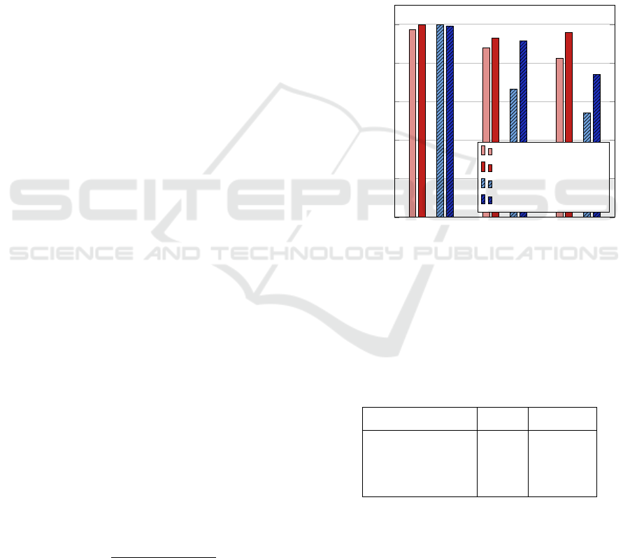
Ds1

P atches

100&200nm

Ds2

P atches

80nm

Ds3

P atches

80nm

0.2

0.4

0.6

0.8

Precision / Recall

F DA

: Precision

CN N −C l

: Precision

F DA

: Recall

CN N −C l

: Recall

Figure 5: Precision and recall of the classiﬁcation results.

Values are given for the positive class. Mostly, precision

is higher than recall, as preferred. The M

CNN-Cl

method

provides stronger results.

Table 2: Classiﬁcation accuracy results for the generated

data sets and the two methods: frequency domain analysis

plus Random Forest classiﬁer M

FDA&RF

and CNN classiﬁ-

cation M

CNN-Cl

.For each row, the bold value shows the best

result.

Data set / method M

FDA

CNN-Cl

Ds1

Patches

100&200nm

0.985 0.995

Ds2

Patches

80nm

0.786 0.922

Ds3

Patches

80nm

0.713 0.854

6 RESULTS AND DISCUSSION

In the following Sections 6.1 and 6.2, we present and

discuss results for the two different classes of experi-

ments that were described in Section 5. Then, we pro-

vide benchmark results for our pipeline in Section 6.3.

Real-time Low SNR Signal Processing for Nanoparticle Analysis with Deep Neural Networks

Table 3: Detection results evaluated for the baseline method and the four presented methods on ﬁve data sets. Quality measures

are given as precision, recall and F

-score. For each row, the bold value shows the best result.

Data set / method M

Baseline

FCN-Det

CNN-Cl

TS-Det

CNN-Cl

Ds4

200nm

Precision 0.909 0.888 0.908 0.933 0.933

Recall 0.787 0.763 0.742 0.903 0.892

-score 0.844 0.821 0.817 0.918 0.918

Ds5

100nm

Precision 0.769 0.814 0.842 0.235 0.938

Recall 0.798 0.857 0.857 0.929 0.803

-score 0.783 0.835 0.810 0.375 0.865

Ds6

80nm

Precision 0.410 0.782 0.877 0.098 0.887

Recall 0.492 0.715 0.677 0.967 0.506

-score 0.448 0.747 0.764 0.177 0.644

Ds7

80nm

Precision 0.330 0.347 0.840 0.025 0.829

Recall 0.549 0.795 0.707 0.967 0.428

-score 0.412 0.483 0.768 0.049 0.564

Ds8

80nm

Precision 0.053 0.258 0.801 0.017 0.729

Recall 0.561 0.782 0.553 0.970 0.355

-score 0.097 0.388 0.655 0.033 0.478

6.1 Standalone Particle Classiﬁcation

The results for the standalone particle classiﬁcation

are shown in Table 2. It shows classiﬁcation accuracy

for the two presented classiﬁcation methods M

FDA

and M

CNN-Cl

We observe nearly the same accuracy of both

motehods on the easier Ds1

Patches

100&200nm

data set. How-

ever, the results on the 80 nm data sets Ds2

Patches

80nm

and

Ds3

Patches

80nm

show that the M

CNN-Cl

method outperforms

the M

FDA

method on harder tasks. The difference in

accuracy between data sets Ds2

Patches

80nm

and Ds3

Patches

80nm

show that transferring the model to a different mea-

surement is possible but leads, in this case, to a sig-

niﬁcant decrease in accuracy. However, we show that

even the transferred classiﬁcation model is able to im-

prove the detection results provided in the next sec-

tion.

For more insight, we also detail precision and re-

call of each approach and data set in Figure 5. In

general, the precision is higher than the recall, which

is also what is preferred most of the time. In addi-

tion, the M

CNN-Cl

method shows better results than

the M

FDA

method in both criteria. All in all, these re-

sults led us to the decision to use the M

CNN-Cl

method

together with our detection networks for our sensor

data experiments that are presented in the following

section.

6.2 Sensor Data Experiment

The results for the sensor data experiment are shown

in Table 3. The quality measures precision, recall and

-score are provided for the baseline method and the

four presented methods on ﬁve data sets. The best

results of each experiment are printed bold.

First, it should be noted that Ds6

80nm

was used to

train the M1

FCN-Det

detector and to extract the training

data for data set Ds3

Patches

80nm

, which was used to train

the applied M

CNN-Cl

classiﬁer. Therefore, the results

of methods M1

FCN-Det

, M2

FCN-Det

CNN-Cl

and M4

TS-Det

CNN-Cl

for

Ds6

80nm

are training scores. The other data sets were

not seen during training and used to calculate the test-

ing score. Since the time-series classiﬁcation network

was trained using synthetic data, all results of method

TS-Det

are test results.

The evaluation shows that nearly all our methods

outperform the baseline method M

Baseline

by a large

margin. The M3

TS-Det

and M4

TS-Det

CNN-Cl

methods provide

strong results on data sets with a median SNR above

one. For data set Ds4

200nm

, the classiﬁer is not even

needed to sort out false positives. For data sets with a

median SNR below one however, the resulting time-

series detection network shows very high sensitivity,

resulting in low precision in order to ﬁnd most true

positives. Therefore, it heavily relies on the classiﬁer

to sort out false positives consisting of noise and arti-

facts. For these data sets, the combination of the FCN

detector and the CNN classiﬁer, method M2

FCN-Det

CNN-Cl

proves to be the strongest method. It achieves a preci-

sion above 0.8 on all three data sets, thus having a low

BIOSIGNALS 2018 - 11th International Conference on Bio-inspired Systems and Signal Processing

number of false positives. This indicates that, espe-

cially for low SNR signals, the local spatial informa-

tion is important to perform reliable detection and that

time-series information of one pixel is not enough to

distinguish between artifact and particle signals. The

recall, despite being not optimal, is sufﬁcient for a

lot of tasks, in which the existence and size distribu-

tions of particles should be derived. The worse results

for this method on data sets Ds4

200nm

and Ds5

100nm

easily explained by the fact that the networks were not

trained with images containing 100 nm and 200 nm

particles.

6.3 Performance Analysis

We proﬁled the proposed processing pipeline as well

as each deep neural network on an NVIDIA GeForce

GTX 1080 Ti. For whole pipeline application, we

achieve 15.296 ms per frame (65.4 fps) when using

the M4

TS-Det

CNN-Cl

method and 23.478 ms (42.5 fps) when

using the M4

TS-Det

CNN-Cl

method. Applying the FCN de-

tector on one image takes 0.827 ms while the time-

series analysis network is slower and takes 9.675 ms.

The classiﬁcation CNN takes 0.119 ms per patch clas-

siﬁcation. All measurements were performed on data

set Ds7

80nm

, which has 6750 images with a resolution

of 880 px × 115 px.

7 CONCLUSIONS

In this work, we proposed additional deep neural net-

work methods for the PAMONO sensor data analy-

sis pipeline. We showed that through this extensions,

the detection of blobs with a median SNR below one

is possible. All in all, we achieved results on sig-

nals with a median SNR of 0.7 that were previously

reached on data sets with a median SNR of 1.25.

Our pipeline, consisting of detection and classiﬁ-

cation networks, was able to achieve sufﬁciently high

results for most real world nanoparticle analysis ap-

plications of the PAMONO sensor while fulﬁlling the

soft real-time property on desktop GPUs. We are able

to successfully analyze suspensions containing 80 nm

polystyrene particles, given our current sensor experi-

ment setup. Detecting even smaller particles in the fu-

ture requires either the improvement of the data (with

higher SNR for the same particle size) or the capa-

bility of the detection pipeline to handle even lower

SNR. In addition, we aim to bring the pipeline to

embedded GPUs, to further move towards the goal

of small, mobile nanoparticle analysis with the PA-

MONO sensor.

ACKNOWLEDGMENTS

This work has been supported by DEUTSCHE

FORSCHUNGSGEMEINSCHAFT (DFG) within the

Collaborative Research Center SFB 876 Providing In-

formation by Resource-Constrained Analysis, project

B2.

REFERENCES

Abadi, M., Agarwal, A., Barham, P., Brevdo, E., Chen, Z.,

Citro, C., Corrado, G. S., Davis, A., Dean, J., Devin,

M., Ghemawat, S., Goodfellow, I., Harp, A., Irving,

G., Isard, M., Jia, Y., Jozefowicz, R., Kaiser, L., Kud-

lur, M., Levenberg, J., Man

e, D., Monga, R., Moore,

S., Murray, D., Olah, C., Schuster, M., Shlens, J.,

Steiner, B., Sutskever, I., Talwar, K., Tucker, P., Van-

houcke, V., Vasudevan, V., Vi

egas, F., Vinyals, O.,

Warden, P., Wattenberg, M., Wicke, M., Yu, Y., and

Zheng, X. (2015). Tensorﬂow: Large-scale machine

learning on heterogeneous systems.

Aljarrah, I., Toma, A., and Al-Rousan, M. (2015). An au-

tomatic intelligent system for diagnosis and conﬁrma-

tion of johne’s disease. Int. J. Intell. Syst. Technol.

Appl., 14(2):128–144.

Beusink, J. B., Lokate, A. M. C., Besselink, G. A. J., Pruijn,

G. J. M., and Schasfoort, R. B. M. (2008). Angle-

scanning spr imaging for detection of biomolecular

interactions on microarrays. Biosensors and Bioelec-

tronics, 23(6):839–844.

Breiman, L. (2001). Random forests. Machine Learning,

45(1):5–32.

Castellano, G., Bonilha, L., Li, L. M., and Cendes, F.

(2004). Texture analysis of medical images. Clinical

Radiology, 59(12):1061–1069.

Cheezum, M. K., Walker, W. F., and Guilford, W. H. (2001).

Quantitative comparison of algorithms for tracking

single ﬂuorescent particles. Biophysical Journal,

81(4):2378–2388.

Chinowsky, T. M., Mactutis, T., Fu, E., and Yager, P. (2004).

Optical and electronic design for a high-performance

surface plasmon resonance imager. In Optical Tech-

nologies for Industrial, Environmental, and Biological

Sensing, pages 173–182.

Dragovic, R. A., Gardiner, C., Brooks, A. S., Tannetta,

D. S., Ferguson, D. J., Hole, P., Carr, B., Redman,

C. W., Harris, A. L., Dobson, P. J., Harrison, P.,

and Sargent, I. L. (2011). Sizing and phenotyping

of cellular vesicles using nanoparticle tracking anal-

ysis. Nanomedicine: Nanotechnology, Biology and

Medicine, 7(6):780 – 788.

Duchi, J., Hazan, E., and Singer, Y. (2011). Adaptive sub-

gradient methods for online learning and stochastic

optimization. Journal of Machine Learning Research,

12(Jul):2121–2159.

Dulbecco, R. (1954). Plaque formation and isolation of pure

lines with poliomylitis viruses. Journal of Experimen-

tal Medicine, 99(2):167–182.

Real-time Low SNR Signal Processing for Nanoparticle Analysis with Deep Neural Networks

Gan, S. D. and Patel, K. R. (2013). Enzyme immunoassay

and enzyme-linked immunosorbent assay. The Jour-

nal of Investigative Dermatology, 133(9):1–3.

Giebel, K.-F., Bechinger, C. S., Herminghaus, S., Riedel,

M., Leiderer, P., Weiland, U. M., and Bastmeyer, M.

(1999). Imaging of Cell/Substrate Contacts of Living

Cells with Surface Plasmon Resonance Microscopy.

Bibliothek der Universit

at Konstanz, Konstanz, Ger-

many.

Gonzalez, R. C. and Woods, R. E. (2006). Digital Image

Processing (3rd Edition). Prentice-Hall, Inc, Upper

Saddle River, NJ, USA.

Hall, M., Frank, E., Holmes, G., Pfahringer, B., Reutemann,

P., and Witten, I. H. (2009). The weka data mining

software: An update. ACM SIGKDD Explorations

Newsletter, 11(1):10–18.

Hecht-Nielsen, R. et al. (1988). Theory of the backpropaga-

tion neural network. Neural Networks, 1(Supplement-

1):445–448.

Iandola, F. N., Moskewicz, M. W., Ashraf, K., Han, S.,

Dally, W. J., and Keutzer, K. (2016). Squeezenet:

Alexnet-level accuracy with 50x fewer parameters and

<1mb model size. CoRR, abs/1602.07360.

Karpathy, A., Toderici, G., Shetty, S., Leung, T., Suk-

thankar, R., and Li, F.-F. (2014). Large-scale video

classiﬁcation with convolutional neural networks. In

2014 IEEE Conference on Computer Vision and Pat-

tern Recognition, CVPR 2014, Columbus, OH, USA,

June 23-28, 2014, pages 1725–1732.

Kingma, D. P. and Ba, J. (2014). Adam: A method for

stochastic optimization. In Proceedings of the 3rd In-

ternational Conference on Learning Representations

(ICLR).

Kohavi, R. (1995). Wrappers for Performance Enhance-

ment and Oblivious Decision Graphs. PhD thesis,

Stanford University, Department of Computer Sci-

ence, Stanford University.

Kretschmann, E. (1971). The determination of the optical

constants of metals by excitation of surface plasmons.

European Physical Journal A, 241(4):313–324.

LeCun, Y., Bengio, Y., et al. (1995). Convolutional net-

works for images, speech, and time series. The

handbook of brain theory and neural networks,

3361(10):1995.

Lenssen, J. E., Shpacovitch, V., and Weichert, F. (2017).

Real-time virus size classiﬁcation using surface plas-

mon pamono resonance and convolutional neural net-

works. In Maier-Hein, K. H., Deserno, T. M., Han-

dels, H., and Tolxdorff, T., editors, Bildverarbeitung

ur die Medizin 2017, Informatik Aktuell, pages 98–

103. Springer, Berlin, Germany and Heidelberg, Ger-

many.

Libuschewski, P. (2017). Exploration of Cyber-Physical

Systems for GPGPU Computer Vision-Based Detec-

tion of Biological Viruses . PhD thesis, TU Dortmund,

Dortmund, Germany.

Liu, J., White, J. M., and Summers, R. M. (2010). Auto-

mated detection of blob structures by hessian analysis

and object scale. In Image Processing (ICIP). 17th

IEEE International Conference on, pages 841–844.

Long, J., Shelhamer, E., and Darrell, T. (2015). Fully con-

volutional networks for semantic segmentation. In

IEEE Conference on Computer Vision and Pattern

Recognition, CVPR 2015, Boston, MA, USA, June 7-

12, 2015, pages 3431–3440.

Moon, W. K., Shen, Y.-W., Bae, M. S., Huang, C.-S., Chen,

J.-H., and Chang, R.-F. (2013). Computer-aided tumor

detection based on multi-scale blob detection algo-

rithm in automated breast ultrasound images. Medical

Imaging. IEEE Transactions on, 32(7):1191–1200.

Naimushin, A. N., Soelberg, S. D., Bartholomew, D. U.,

Elkind, J. L., and Furlong, C. E. (2003). A portable

surface plasmon resonance (spr) sensor system with

temperature regulation. Sensors and Actuators B:

Chemical, 96(1-2):253–260.

Pattnaik, P. (2005). Surface plasmon resonance: Applica-

tions in understanding receptor-ligand interaction. Ap-

plied Biochemistry and Biotechnology, 126(2):79–92.

Powers, D. M. W. (2011). Evaluation: From precision, re-

call and f-measure to roc., informedness, markedness

& correlation. Journal of Machine Learning Tech-

nologies, 2(1):37–63.

Scarano, S., Ermini, M. L., Mascini, M., and Minunni,

M. (2011). Surface plasmon resonance imaging for

afﬁnity-based sensing: An analytical approach. In

BioPhotonics. International Workshop on, pages 957–

966.

Shpacovitch, V., Temchura, V., Matrosovich, M.,

Hamacher, J., Skolnik, J., Libuschewski, P., Siedhoff,

D., Weichert, F., Marwedel, P., M

uller, H.,

Uberla, K.,

Hergenr

oder, R., and Zybin, A. (2015). Application

of surface plasmon resonance imaging technique for

the detection of single spherical biological submi-

crometer particles. Analytical Biochemistry: Methods

in the Biological Sciences, 486:62–69.

Siedhoff, D. (2016). A parameter-optimizing model-based

approach to the analysis of low-snr image sequences

for biological virus detection. phd, Universit

at Dort-

mund. Publikation.

Siedhoff, D., Libuschewski, P., Weichert, F., Zybin, A.,

Marwedel, P., and M

uller, H. (2014). Modellierung

und optimierung eines biosensors zur detektion viraler

strukturen. In Deserno, T. M., Handels, H., Meinzer,

H.-P., and Tolxdorff, T., editors, Bildverarbeitung f

die Medizin (BVM), Informatik Aktuell, pages 108–

113. Springer, Berlin, Germany and Heidelberg, Ger-

many.

Smal, I., Loog, M., Niessen, W., and Meijering, E. (2009).

Quantitative comparison of spot detection methods

in live-cell ﬂuorescence microscopy imaging. In

Biomedical Imaging: From Nano to Macro. IEEE In-

ternational Symposium on, pages 1178–1181.

Steiner, G. and Salzer, R. (2001). Biosensors based on spr

imaging. In T

ubingen, U., editor, 2. BioSensor Sym-

posium, T

ubingen, Germany. Universit

at T

ubingen.

Szegedy, C., Liu, W., Jia, Y., Sermanet, P., Reed, S.,

Anguelov, D., Erhan, D., Vanhoucke, V., and Rabi-

novich, A. (2015). Going deeper with convolutions.

In IEEE Conference on Computer Vision and Pattern

Recognition (CVPR), pages 1–9. IEEE.

BIOSIGNALS 2018 - 11th International Conference on Bio-inspired Systems and Signal Processing

Woodward, R. M., Wallace, V. P., Arnone, D. D., Linﬁeld,

E. H., and Pepper, M. (2003). Terahertz pulsed imag-

ing of skin cancer in the time and frequency domain.

Journal of Biological Physics, 29(2-3):257–259.

Zybin, A. (2010). DE patent 10,2009,003,548 A1: Ver-

fahren zur hochaufgel

osten erfassung von nanopar-

tikeln auf zweidimensionalen messﬂ

achen.

Zybin, A. (2013). US patent 8,587,786 B2: Method

for high-resolution detection of nanoparticles on two-

dimensional detector surfaces.

Real-time Low SNR Signal Processing for Nanoparticle Analysis with Deep Neural Networks