Deep Learning Techniques for Classification of P300 Component
Ji
ˇ
r
´
ı Van
ˇ
ek and Roman Mou
ˇ
cek
Department of Computer Science and Engineering, University of West Bohemia, Plzen, Czech Republic
Keywords:
Deep Learning, Neural Networks, Stacked Autoencoder, Deep Belief Networks, Classification, Event-related
Potentials, P300 Component.
Abstract:
Deep learning techniques have proved to be beneficial in many scientific disciplines and have beaten state-
of-the-art approaches in many applications. The main aim of this article is to improve the success rate of
deep learning algorithms, especially stacked autoencoders, when they are used for detection and classifica-
tion of P300 event-related potential component that reflects brain processes related to stimulus evaluation or
categorization. Moreover, the classification results provided by stacked autoencoders are compared with the
classification results given by other classification models and classification results provided by combinations
of various types of neural network layers.
1 INTRODUCTION
Brain-computer interface (BCI) is a method of com-
munication based on neural activity generated by
the brain and it is independent of its normal output
pathways of peripheral nerves and muscles (Valla-
bhaneni et al., 2005). A big advantage of this ap-
proach is a possibility to record BCI activity non-
invasively using the techniques of electroencephalo-
graphy (EEG) and event-related potentials (ERPs).
The technique of event-related potentials is then ba-
sed on the elicitation and detection of so called event-
related (evoked) components that represent the brain
activity occurring in the EEG signal in a certain time
window after the stimulus onset. Since the correct
detection and classification of evoked components is
not a simple issue, a number of techniques have been
proposed and used for this task.
This work builds on the results of the research
described in the article ’Application of Stacked Au-
toencoders to P300 Experimental Data’ (Va
ˇ
reka et al.,
2017) where the idea of using stacked autoenco-
ders for detection and classification of human brain
activity represented by electroencephalographic and
event-related potential data was presented.
The main goal of this article is to improve the
success rate of stacked autoencoders for the detection
and classification of the P300 component (the most
important and well described cognitive component
occurring in the EEG signal as a response to visual
or audio stimulation), compare the classification re-
sults of stacked autoencoders with the classification
results of other classification models and classifica-
tion results provided by combinations of various types
of neural network layers.
Successful results of such classification approa-
ches could be subsequently used for developing an
evaluation tool that would be suitable for the P300
component detection and classification in many ap-
plications.
The experimental data from the ’Guess the num-
ber experiment’ that is described in (Va
ˇ
reka et al.,
2017) are used for the detection and classification
task; this experimental design is also used as an ex-
ample of the P300 BCI system.
The article is organized as follows. Short descrip-
tions of the P300 component, deep learning approach,
stacked autoencoders, multilayer perceptron and deep
belief networks are provided in Section 2. The ’Guess
the Number’ experiment together with the ’Guess the
number’ application are described in Section 3. The
processing methods and network configurations used
for the detection and classification of the P300 com-
ponent are listed in Section 4. The last two sessions
include the presentation of the results and concluding
discussion.
446
Van
ˇ
ek, J. and Mou
ˇ
cek, R.
Deep Learning Techniques for Classification of P300 Component.
DOI: 10.5220/0006594104460453
In Proceedings of the 11th International Joint Conference on Biomedical Engineering Systems and Technologies (BIOSTEC 2018) - Volume 5: HEALTHINF, pages 446-453
ISBN: 978-989-758-281-3
Copyright © 2018 by SCITEPRESS – Science and Technology Publications, Lda. All rights reserved

2 THEORETICAL BACKGROUND
2.1 P300 Component
Brain Computer Interfaces mostly rely on the de-
tection of the P300 component that is hidden in the
record of human brain activity when the techniques
of electroencephalography and of event-related po-
tentials are used. This component usually occurs in
the EEG signal from 200 ms to 500 ms after stimu-
lus onset. An example of the P300 component in the
EEG signal for common and rare stimuli is given in
Figure 1.
Pz
-200 200 400 600
Time [ms]
6.8
13.5
20.3
27
non-target target
Figure 1: Comparison of averaged EEG responses to com-
mon (non-target) stimuli (Xs) and rare (target) stimuli
(Os). There is a P300 component following the Os sti-
muli (Va
ˇ
reka and Mautner, 2017).
It is very important for practical use that a P300-
based BCI is an effective and straightforward system
that does not require any special training of the user.
2.2 Deep Learning
Deep learning generally allows computational models
that are composed of multiple processing layers to le-
arn representations of data with multiple levels of ab-
straction. These methods have dramatically improved
the state-of-the-art in many scientific disciplines, for
example in speech recognition, visual object recogni-
tion, object detection and many other domains such
as drug discovery and genomics (LeCun et al., 2015).
Deep learning discovers structures in large data
sets by using the backpropagation algorithm to in-
dicate how a machine should change its internal pa-
rameters that are used to compute the representation
in each layer from the representation in the previous
layer (LeCun et al., 2015).
Deep learning has been also widely used in the
EEG field. In (An et al., 2014) a deep learning algo-
rithm was applied to classify EEG data based on mo-
tor imagery task. (Tabar and Halici, 2016) used con-
volutional neural networks and stacked autoencoders
to improve classification performance of EEG motor
imagery signals. (Antoniades et al., 2016) described
a deep learning approach for automatic feature gene-
ration from epileptic intracranial EEG records. (La-
whern et al., 2016) focused on a generalized neural
network architecture that can classify EEG signals in
different BCI tasks. (Stober et al., 2015) compared
several strategies for learning discriminative features
from electroencephalography (EEG) recordings using
deep learning techniques and evaluated them using
the Open–MIIR dataset of EEG recordings. (Grea-
ves, 2014) used recurrent neural networks for classi-
fication of the EEG signal when people were viewing
2D and 3D images. (Jirayucharoensak et al., 2014)
tested a stacked autoencoder using hierarchical fea-
ture learning approach for recognition of EEG-based
emotion. An overview of capabilities of deep neu-
ral architectures for classifying brain signals is given
in (Bozhkov, 2016).
2.3 Stacked Denoising Autoencoders
Stacked Denoising Autoencoder (SDAE) is a variant
of the basic autoencoder. A denoising autoencoder
(DAE) is trained to reconstruct a clean repaired input
from a corrupted version of it (Vincent et al., 2010).
This is beneficial for our classification case because
most of the EEG signal is influenced by noise. How
this denoising works is described in Figure 2.
Figure 2: Stacking denoising autoencoders. After trai-
ning a first level denoising autoencoder its learnt enco-
ding function f
0
is used on the clean input (left). The re-
sulting representation is used to train a second level denoi-
sing autoencoder (middle) to learn a second level encoding
function f
(2)
0
. From there, the procedure can be repeated
(right) (Vincent et al., 2010).
2.4 Multilayer Perceptron
A multilayer perceptron (MLP) is a feed-forward ar-
tificial neural network model that maps sets of input
data onto a set of appropriate outputs. An MLP con-
sists of multiple layers of nodes in a directed graph,
with each layer fully connected to the next one. Ex-
cept for the input nodes, each node is a neuron with
a nonlinear activation function.
2.5 Deep Belief Networks (DBN)
Invented by Geoff Hinton, a Restricted Boltzmann
machine (RBM) is an algorithm useful for dimensi-
onality reduction, classification, regression, collabo-
rative filtering, feature learning and topic modeling.
RBMs are shallow, two-layer neural networks that
constitute the building blocks of deep-belief net-
works. The first layer of the RBM is called the visible
or input layer, the second layer is called the hidden
layer.
Deep Learning Techniques for Classification of P300 Component
447

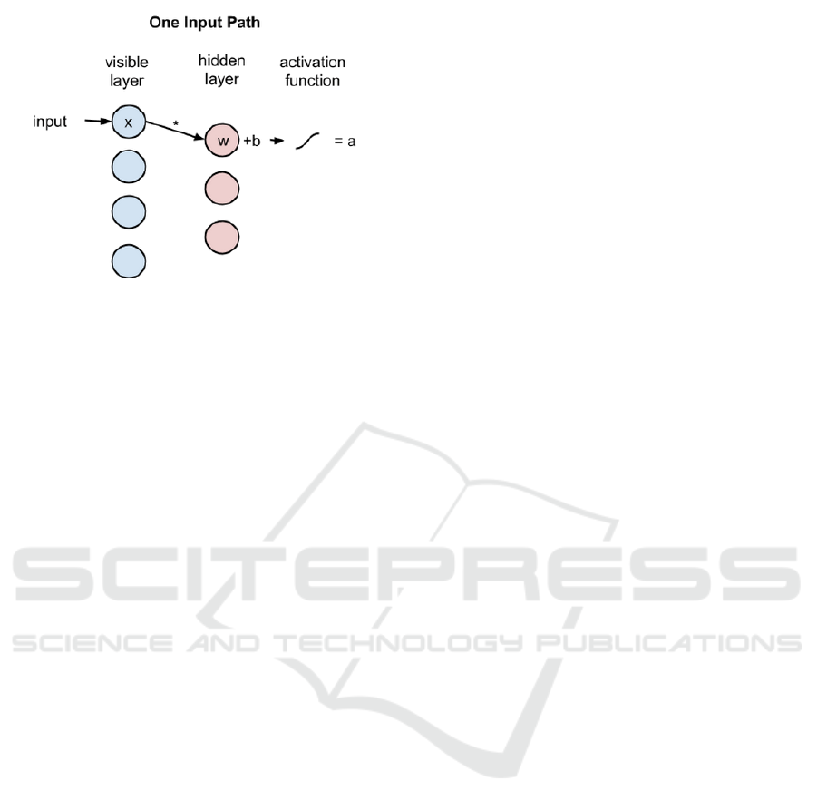
Figure 3: Restricted Boltzmann machine. Visible and hid-
den layers. (Deeplearning4j Development Team, 2017).
Each circle shown in the graph in Figure 3 repre-
sents a neuron-like unit called a node, and nodes are
simply places where calculations take place. The no-
des are connected to each other across layers, but no
two nodes of the same layer are linked.
There is no intra-layer communication - this is the
restriction in a restricted Boltzmann machine. Each
node is a locus of computation that processes in-
put, and begins by making stochastic decisions about
whether to transmit that input or not.
3 EXPERIMENT
The ’Guess the number’ experiment has been desig-
ned and implemented to demonstrate advantages of
the P300 BCI system to the public. The experiment
uses visual stimulation. At first, each participant se-
cretly chooses one number between 1 and 9 on which
he/she concentrates when the numbers from 1 to 9 are
randomly shown on the screen. The EEG signal and
stimuli markers are recorded during the experiment.
The number assumed the participant had chosen
was guessed automatically by an on-line classifier and
manually by a human expert watching and evaluating
the brain event-related potentials of the participant on
the screen. At the end of the experiment the thought
number was verified by asking the participant to re-
veal it.
3.1 Guess the Number Application
The automatic classifier has been developed as a desk-
top Java application for analysis of event-related po-
tential components from the ’Guess the number’ ex-
periment. This application enables its users to classify
event-related components occurring in the EEG sig-
nal off-line (when all data have been collected) or on-
line (data are streamed during the experiment). The
off-line classification mode allows users to test a va-
riety of preprocessing, features extraction and classi-
fication algorithms.
4 P300 DETECTION AND
CLASSIFICATION
4.1 Preprocessing and Feature
Extraction
The same experimental data sets as described in the
article (Va
ˇ
reka et al., 2017) were used in the task.
Since also the same algorithms and settings were used
during the preprocessing phase, the results of the final
classification task are comparable.
• Channel selection: The channels Fz, Cz and Pz
were selected.
• Epoch extraction: The raw EEG signal was split
into segments with the fixed length of 1000 ms.
• Baseline correction: The average of 100 ms in-
terval before each epoch was subtracted from the
whole epoch.
• Interval selection: Only an appropriate time inter-
val (when the P300 component commonly occurs)
was selected in each epoch. The length of the in-
terval was 512 ms and started 175 ms after begin-
ning of each epoch (Va
ˇ
reka et al., 2017).
• Discrete wavelet transformation was used for fea-
ture extraction (Va
ˇ
reka et al., 2017).
• Vector normalizing: Feature vectors were nor-
malized to contain only the samples between -1
and 1.
4.2 Classification
The preprocessed data were split into two parts, trai-
ning and testing datasets. The training dataset con-
tains the data from 13 subjects. The subjects were se-
lected manually based on their P300 response to target
stimuli (Va
ˇ
reka et al., 2017). It is the data from the
same 13 subjects that were described and processed
in the article ’Application of Stacked Autoencoders
to P300 Experimental Data’.
Several types of neural networks are compared
in this paper. All of them are implemented using
the Deeplearning4j library in version 0.8. This is
an open-source distributed deep learning library for
the JVM (Deeplearning4j Development Team, 2017).
HEALTHINF 2018 - 11th International Conference on Health Informatics
448

A specific configuration of each neural network that
was used for classification purposes is dependent on
the type of the network.
The configuration settings of the neural net-
works were determined automatically by an automa-
ted script and only the network configurations pro-
viding the best results (after running 100 tests) were
tested furthermore. The initial configuration was ta-
ken over from (Va
ˇ
reka et al., 2017). The sizes of the
networks were adjusted manually.
A list of configurations is provided in individual
subsections listed bellow. The options avoiding over-
training, early stopping and dropout were used. Also
several combinations of different neural network ty-
pes were tested.
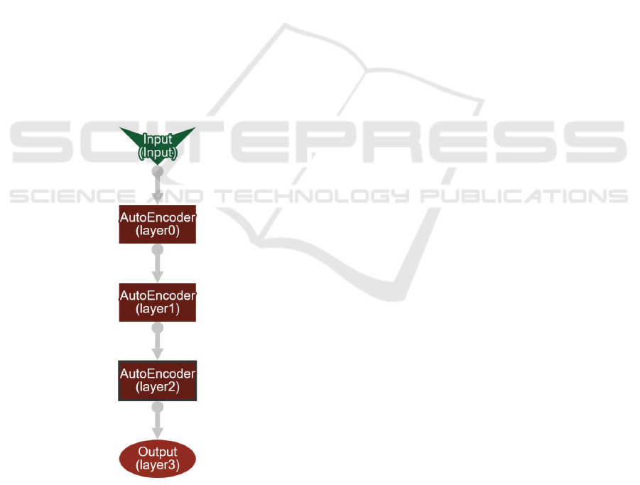
4.3 Classification Settings
All the networks used are composed of several types
of layers. The output layer is the same for all net-
works, the only difference that can be found in the
output layer is the number of its inputs that depends
on the number of outputs of a previous layer. The
scheme of the SDAE networks configuration can be
found in Figure 4.
Figure 4: Stacked Denoising Autoencoders layers configu-
ration. The picture was generated using the Deeplearning4J
web user interface.
To understand the process of setting the neural
networks configurations some terms and procedures
related to the neural networks used and Deeplear-
ning4j library are explained. The learning rate, or step
rate, is the rate at which a function steps through the
search space. Smaller steps result in longer training
times, but can lead to more precise results.
An epoch is defined as a full pass of the data
set. An iteration in the Deeplearning4J library is defi-
ned as the number of parameter updates in a row, for
each minibatch (Deeplearning4j Development Team,
2017).
Momentum is an additional factor in determining
how fast an optimization algorithm converges to the
optimum point. Momentum, also known as Neste-
rov’s momentum, influences the speed of learning. It
causes the model to converge faster to a point of mi-
nimal error. Momentum adjusts the size of the next
step, the weight update, based on the previous steps
gradient (Deeplearning4j Development Team, 2017).
The Deeplearning4j library supports several diffe-
rent types of weight initializations that could be chan-
ged with the weightInit parameter. Also the seed pa-
rameter is supported but in this case it was not used to
minimize nondeterministic behavior of network initi-
alization.
Dropout is used for regularization in neural net-
works. Like all regularization techniques, its purpose
is to prevent over-fitting. Dropout randomly makes
nodes in the neural network drop out by setting them
to zero, which encourages the network to rely on ot-
her features that act as signals. That, in turn, creates
more generalizable representations of data (Srivastava
et al., 2014).
Activation, or the activation function, in the dom-
ain of neural networks is defined as the mapping of the
input to the output via a non-linear transform function
at each ’node’, which is simply a locus of computa-
tion within the net. Each layer in a neural net consists
of many nodes, and the number of nodes in a layer
is known as its width (Deeplearning4j Development
Team, 2017).
Backpropagation is a repeated application of the
chain rule of calculus for partial derivatives. The first
step is to calculate the derivatives of the objective
function with respect to the output units, then the de-
rivatives of the output of the last hidden layer to the
input of the last hidden layer (LeCun et al., 2012).
The retrain parameter was turned off and the back
propagation parameter was turned on in all cases. The
list of the used networks together with their configu-
rations follows.
4.3.1 SDAE - Smaller Size
• Number of iterations: 3500
• Number of layers: 4
Deep Learning Techniques for Classification of P300 Component
449

• Learning rate: 0.05
• Size of layers: First - Input 48 Output 48; Second
- Input 48 Output 24; Third - Input 24 Output 12;
Fourth - Input 12 Output 2
• Weight Initialization: Rectified linear unit
• Activation Function: Leaky Rectified linear unit
• Dropout: 0.5
• Lossfunction: Multiclass Cross Entropy
• Corruption: First layer: 0.1
• Output layer: Activation Softmax, Weight Initia-
lization Xavier, Lossfunction Negative Log Like-
lihood
4.3.2 SDAE - Bigger Size
• Number of iterations: 3500
• Number of layers: 4
• Learning rate: 0.05
• Size of layers: First - Input 48 Output 48; Second
- Input 48 Output 48; Third - Input 48 Output 24;
Fourth - Input 24 Output 2
• Weight Initialization: Rectified linear unit
• Activation Function: Leaky Rectified linear unit
• Dropout: 0.5
• Lossfunction: Multiclass Cross Entropy
• Corruption: First layer: 0.1
• Output layer: Activation Softmax, Weight Initia-
lization Xavier, Lossfunction Negative Log Like-
lihood
4.3.3 SDAE with Higher Corruption
• Number of iterations: 3500
• Number of layers: 4
• Learning rate: 0.05
• Size of layers: First - Input 48 Output 48; Second
- Input 48 Output 48; Third - Input 48 Output 24;
Fourth - Input 24 Output 2
• Weight Initialization: Rectified linear unit
• Activation Function: Leaky Rectified linear unit
• Dropout: 0.5
• Lossfunction: Multiclass Cross Entropy
• Corruption: First layer: 0.2
• Output layer: Activation Softmax, Weight Initia-
lization Xavier, Lossfunction Negative Log Like-
lihood
4.3.4 SDAE with no Corruption
• Number of iterations: 3500
• Number of layers: 4
• Learning rate: 0.05
• Size of layers: First - Input 48 Output 48; Second
- Input 48 Output 48; Third - Input 48 Output 24;
Fourth - Input 24 Output 2
• Weight Initialization: Rectified linear unit
• Activation Function: Leaky Rectified linear unit
• Dropout: 0.5
• Lossfunction: Multiclass Cross Entropy
• Corruption: First layer: 0.0
• Output layer: Activation Softmax, Weight Initia-
lization Xavier, Lossfunction Negative Log Like-
lihood
4.3.5 Multilayer Perceptron (MLP)
• Number of iterations: 3000
• Number of layers: 3
• Learning rate: 0.003
• Size of layers: First - Input 48 Output 100; Second
- Input 100 Output 50; Third - Input 50 Output 2
• Weight Initialization: Rectified linear unit
• Activation Function: Rectified linear unit
• Dropout: 0.6
• Updater: Nesterov’s momentum: 0.9
• Output layer: Activation Softmax, Lossfunction -
Negative Log Likelihood
4.3.6 Deep Belief Network (DBN)
• Number of iterations: 2500
• Number of layers: 3
• Size of layers: First - Input 48 Output 120; Second
- Input 120 Output 45; Third - Input 45 Output 2
• Updater: Stochastic Gradient Descent
• Activation Function: Default
• Dropout: 0
• Lossfunction: Multiclass Cross Entropy, Squared
Loss
• Output Layer: Lossfunction Multiclass Cross En-
tropy, Activation Softmax
HEALTHINF 2018 - 11th International Conference on Health Informatics
450

4.3.7 Mixed Neural Network
• Number of iterations: 3000
• Number of layers: 4
• Learning rate: 0.005
• Type of layers: SDAE, DBN, SDAE, Output layer
• Size of layers: First - Input 48 Output 128; Second
- Input 128 Output 256; Third - Input 256 Output
128; Fourth - Input 128 Output 2
• Weight Initialization: Rectified linear unit
• Activation Function: Rectified linear unit
• Corruption: First layer: 0.1
• Dropout: 0.5
• Updater: Nesterov’s momentum 0.9
• Regularization: True
• Lossfunction: Cross Entropy: Binary Classifica-
tion
• Output Layer: Activation Softmax, Weight Initia-
lization Xavier
4.3.8 Mixed Neural Network 2
• Number of iterations: 3000
• Number of layers: 4
• Learning rate: 0.005
• Type of layers: SDAE, DBN, RBN, Output layer
• Size of layers: First - Input 48 Output 128; Second
- Input 128 Output 256; Third - Input 256 Output
128; Fourth - Input 128 Output 2
• Weight Initialization: Rectified linear unit
• Activation Function: Rectified linear unit
• Corruption: First layer: 0.1, Second layer: 0.1
• Dropout: 0.5
• Updater: Nesterov’s momentum 0.9
• Regularization: True
• Lossfunction: Cross Entropy: Binary Classifica-
tion
• Output Layer: Activation Softmax, Weight Initia-
lization Xavier
4.3.9 Mixed Neural Network 3
• Number of iterations: 3000
• Number of layers: 4
• Learning rate: 0.005
• Type of layers: SDAE, SDAE, RBN, Output layer
• Size of layers: First - Input 48 Output 64; Second
- Input 64 Output 128; Third - Input 128 Output
128; Fourth - Input 128 Output 2
• Weight Initialization: Rectified linear unit
• Activation Function: Rectified linear unit
• Dropout: 0.5
• Corruption: First layer: 0.1
• Updater: Nesterov’s momentum 0.9
• Regularization: True
• Lossfunction: Cross Entropy: Binary Classifica-
tion
• Output Layer: Activation Softmax, Weight Initia-
lization Xavier
4.3.10 Early Stopping
Some of networks settings were also tested using the
early stopping criterion instead of dropout. In these
cases dropout was set to 0 and the early stopping cri-
terion was set to the number of epochs with no im-
provement in the value of the classification success
rate (the number of epochs with no improvement was
set to 7 epochs). The threshold for the minimal im-
provement that was considered as a real improvement
was also set, its value was adjusted with respect to the
learning rate and updater settings.
5 RESULTS
Average classification success rates and also the best
and the worst classification success rates were com-
puted for all tested classification methods. Be-
cause training of neural networks is generally non-
deterministic, all classification tasks were run (trained
and evaluated) for at least 1000 times.
The results are provided in Table 1. The neural
networks used for the classification task (the whole
specification of them is available in Section 4.3) are
listed in the first column. The average success rate
is provided in the second column, while maximum
success rate and minimum success rate are stated in
the third and fourth columns respectively. The num-
ber of runs from which all previous numbers were cal-
culated is given in the last column. The results from
the same experiment using the same data but diffe-
rent network settings and provided within the article
’Application of Stacked Autoencoders to P300 Expe-
rimental Data’ (Va
ˇ
reka et al., 2017) are available be-
low the first double horizontal line.
Deep Learning Techniques for Classification of P300 Component
451

Table 1: Classification results - average, maximum and minimum success rates and number of runs.
Method Average Minimum Maximum Number of Runs
SDAE small 74.44 66.02 79.13 3339
SDAE big 74.65 61.65 80.10 4051
SDAE big with 0.2 corrupt 74.59 66.99 80.10 4939
SDAE with no corruption 74.58 66.50 79.61 5541
SDAE E.Stop 73.78 64.08 79.12 5848
MLP 72.52 64.56 79.62 3195
MLP E.Stop 72.86 65.05 77.67 3380
Mixed neural network 73.05 65.54 79.61 2378
Mixed neural network 3 73.24 63.53 80.10 2090
Mixed neural network 2 73.17 66.50 78.64 2029
Mixed neural network E.Stop 72.78 67.47 78.64 2071
DBN 72.41 66.02 77.19 2516
DBN E.Stop 72.94 36.41 78.15 2212
SDA (Va
ˇ
reka et al., 2017) 74.00 - 79.38 400
MLP (Va
ˇ
reka et al., 2017) 68.94 - 76.70 400
Bayesian LDA (Va
ˇ
reka et al., 2017) 73.65 - 77.16 400
Linear discriminant analysis (Va
ˇ
reka et al., 2017) 68.77 - 75.63 400
Support vector machines (Va
ˇ
reka et al., 2017) 65.43 - 73.71 400
Human expert (Va
ˇ
reka et al., 2016) 64.43
Table 1 shows that the best results are provided by
the networks with stacked denoising autoencoder lay-
ers followed by the networks with combined types of
layers (but also including SDAEs). Also the neural
network examples where the early stopping was not
applied show a better result for the network with stac-
ked denoising autoencoder layers, but only thanks to
the experimentally determined number of iterations.
The best results thus show only the networks with
SDAE layers (more specifically with three SDAE lay-
ers since the networks with more SDAE layers were
not tested) and with bigger size of layers (in compa-
rison with other SDAE networks). The setting of the
corruption parameter had also a small impact on the
classification success rate.
6 DISCUSSION AND FUTURE
WORK
There are many possible combinations of neural net-
works, types and sizes of their layers, and their ot-
her adjustable criteria that influence the classification
success rate. Within this work only a few combina-
tions of layers and settings promising a possible high
classification success rate were tested. Not all of these
combinations seem to be beneficial for future long-
term testing but some of them have been chosen for
the next processing since they have provided better
results than the human expert who detected and clas-
sified the P300 component on-line. If trained in ad-
vance most of the described neural networks are ca-
pable to perform the presented classification task on-
line.
A big impact on the classification results had over-
training of the networks that was minimized by pro-
per setting of the early stopping or dropout criterion.
Another possible solution could be to get a bigger
training sample or a different training set that could
prevent the networks from over-training. Also further
experiments with searching the best dropout or early
stopping criterion could improve the classification re-
sults.
Also other network settings could improve the
classification success rate, e.g. the size of the network
layers influences the classification success rate but
also computational complexity significantly. A com-
bination of more types of networks or changes in the
order of the used neural networks seem to also be be-
neficial approaches. In comparison to the original ex-
periments (Va
ˇ
reka et al., 2017) the better results pre-
sented in this article have been achieved thanks to ad-
justments of the used networks and their layers set-
tings.
ACKNOWLEDGEMENTS
This publication was supported by the UWB grant
SGS-2016-018 Data and Software Engineering for
Advanced Applications.
HEALTHINF 2018 - 11th International Conference on Health Informatics
452

REFERENCES
An, X., Kuang, D., Guo, X., Zhao, Y., and He, L. (2014).
A Deep Learning Method for Classification of EEG
Data Based on Motor Imagery, pages 203–210. Sprin-
ger International Publishing, Cham.
Antoniades, A., Spyrou, L., Took, C. C., and Sanei, S.
(2016). Deep learning for epileptic intracranial eeg
data. In 2016 IEEE 26th International Workshop on
Machine Learning for Signal Processing (MLSP), pa-
ges 1–6.
Bozhkov, L. (2016). Overview of deep learning architectu-
res for classifying brain signals. In KSI Transactions
on Knowledge Society, volume IX, pages 54–59. Kno-
wledge Society Institute.
Deeplearning4j Development Team (2017). Deeplear-
ning4j: Open-source distributed deep learning for the
JVM, Apache Software Foundation License 2.0. [on-
line] available at: http://deeplearning4j.org [Accessed
20 Feb. 2017].
Greaves, A. S. (2014). Classification of EEG with recurrent
neural networks.
Jirayucharoensak, S., Pan-Ngum, S., and Israsena, P.
(2014). EEG-based emotion recognition using deep
learning network with principal component based co-
variate shift adaptation. The Scientific World Journal,
2014.
Lawhern, V. J., Solon, A. J., Waytowich, N. R., Gordon,
S. M., Hung, C. P., and Lance, B. J. (2016). Eegnet: A
compact convolutional network for eeg-based brain-
computer interfaces. CoRR, abs/1611.08024.
LeCun, Y., Bengio, Y., and Hinton, G. (2015). Deep lear-
ning. Nature, 521(7553):436–444.
LeCun, Y. A., Bottou, L., Orr, G. B., and M
¨
uller, K.-
R. (2012). Efficient backprop. In Neural networks:
Tricks of the trade, pages 9–48. Springer.
Srivastava, N., Hinton, G., Krizhevsky, A., Sutskever, I.,
and Salakhutdinov, R. (2014). Dropout: A simple way
to prevent neural networks from overfitting. The Jour-
nal of Machine Learning Research, 15(1):1929–1958.
Stober, S., Sternin, A., Owen, A. M., and Grahn, J. A.
(2015). Deep feature learning for EEG recordings.
arXiv preprint arXiv:1511.04306.
Tabar, Y. R. and Halici, U. (2016). A novel deep learning
approach for classification of EEG motor imagery sig-
nals. Journal of neural engineering, 14(1):016003.
Vallabhaneni, A., Wang, T., and He, B. (2005). Braincom-
puter interface. In Neural engineering, pages 85–121.
Springer.
Va
ˇ
reka, L., Prokop, T., Mou
ˇ
cek, R., Mautner, P., and
ˇ
St
ˇ
ebet
´
ak, J. (2017). Application of Stacked Autoen-
coders to P300 Experimental Data, pages 187–198.
Springer International Publishing, Cham.
Va
ˇ
reka, L. and Mautner, P. (2017). Stacked autoencoders
for the P300 component detection. Frontiers in Neu-
roscience, 11:302.
Va
ˇ
reka, L., Prokop, T.,
ˇ
St
ˇ
ebet
´
ak, J., and Mou
ˇ
cek, R. (2016).
Guess the number - applying a simple brain-computer
interface to school-age children. In Proceedings of
the 9th International Joint Conference on Biomedi-
cal Engineering Systems and Technologies - Volume
4: BIOSIGNALS, (BIOSTEC 2016), pages 263–270.
INSTICC, ScitePress.
Vincent, P., Larochelle, H., Lajoie, I., Bengio, Y., and
Manzagol, P.-A. (2010). Stacked denoising autoen-
coders: Learning useful representations in a deep net-
work with a local denoising criterion. J. Mach. Learn.
Res., 11:3371–3408.
Deep Learning Techniques for Classification of P300 Component
453