Hierarchical Reinforcement Learning for Real-Time Strategy Games

Remi Niel

, Jasper Krebbers

, Madalina M. Drugan

and Marco A. Wiering

Institute of Artiﬁcial Intelligence and Cognitive Engineering, University of Groningen, The Netherlands

ITLearns.Online, The Netherlands

Keywords:

Computer Games, Reinforcement Learning, Multi-agent Systems, Multi-layer Perceptrons, Real-Time

Strategy Games.

Abstract:

Real-Time Strategy (RTS) games can be abstracted to resource allocation applicable in many ﬁelds and indus-

tries. We consider a simpliﬁed custom RTS game focused on mid-level combat using reinforcement learning

(RL) algorithms. There are a number of contributions to game playing with RL in this paper. First, we combine

hierarchical RL with a multi-layer perceptron (MLP) that receives higher-order inputs for increased learning

speed and performance. Second, we compare Q-learning against Monte Carlo learning as reinforcement learn-

ing algorithms. Third, because the teams in the RTS game are multi-agent systems, we examine two different

methods for assigning rewards to agents. Experiments are performed against two different ﬁxed opponents.

The results show that the combination of Q-learning and individual rewards yields the highest win-rate against

the different opponents, and is able to defeat the opponent within 26 training games.

1 INTRODUCTION

Games are a thriving area for reinforcement learning

(RL) which have a long and mutually beneﬁcial re-

lationship (Szita, 2012). Evolution Chamber for ex-

ample uses an evolutionary algorithm to ﬁnd build-

orders in the game of Starcraft 2. Temporal-difference

learning, Monte Carlo learning and evolutionary RL

(Wiering and Van Otterlo, 2012) are among the most

popular techniques within the RL approach to games

(Szita, 2012). Most RL research is based on the

Markov decision process (MDP) that is a sequential

decision making problem for fully observed worlds

with the Markov property (Markov, 1960). Many

RL techniques use MDPs as learning problems with

stochastic nature; in multi-agent systems (Littman,

1994) the environment is also non-stationary.

As an alternative to RL, the AI opponents in to-

day’s games work mostly via ﬁnite state machines

(FSMs) which cannot develop new strategies and are

thus predictable. A higher difﬁculty is usually mod-

elled by increasing gather-, attack- and hit-point mod-

iﬁers of AI (Buro et al., 2007). The FSM behaviour

is solely based on ﬁxed state-transition tables. There-

fore, in the past dynamic scripting has been proposed

which can optimize performance and therefore the

challenge (Spronck et al., 2006), but it is still depen-

dent on a pre-programmed rule-base.

The real-time strategy (RTS) genre is a game

played in real-time, where both players make moves

simultaneously. Moves in RTS games can generally

be seen as actions, such as move to a certain posi-

tion, attack a speciﬁc unit, construct this building etc.

These actions can be performed by units which are

semi-autonomous agents. These agents come in dif-

ferent types with their own attributes and actions they

can perform. The player can control all agents that are

on his/her team via mouse and keyboard. The game

environment is often seen from above with an angle

that shows depth, and teams are indicated by colour.

The RTS genre is a particularly hard nut to crack

for RL. In RTS games, the game-play consists of

many different game-play components like resource

gathering, unit building, scouting, planning and com-

bat, which have to be handled in parallel in order to

win (Marthi et al., 2005). In this paper we propose

the use of hierarchical reinforcement learning (HRL)

that allows RL to scale up to more complex problems

(Barto and Mahadevan, 2003) to play an RTS game.

Hierarchical reinforcement learning allows for a di-

vide and conquer strategy (van Seijen et al., 2017),

which signiﬁcantly simpliﬁes the learning problem.

Towards the top of the hierarchy, the problem con-

sist of selecting the best macro actions that take more

than a single time step. The Semi-Markov decision

process (SMDP) theory for HRL allows for actions

470

Niel, R., Krebbers, J., Drugan, M. and Wiering, M.

Hierarchical Reinforcement Learning for Real-Time Strategy Games.

DOI: 10.5220/0006593804700477

In Proceedings of the 10th International Conference on Agents and Artiﬁcial Intelligence (ICAART 2018) - Volume 2, pages 470-477

ISBN: 978-989-758-275-2

that last multiple time steps (Puterman, 1994).

Our RTS approach focusses on the sub-process

of mid-level combat strategy. Neural network im-

plementations of low-level combat behaviour have al-

ready shown reasonable results in (Patel, 2009; Buro

and Churchill, 2012). Agents in the game of Counter

Strike were given a single task and a neural network

was used to optimize performance accomplishing this

task. Our method uses task selection: instead of giv-

ing the neural network a single task for which it has to

optimize, our neural network optimizes task selection

for each unit. The unit then executes an order, like

defend the base or attack that unit. The implementa-

tion of the behavior is executed via an FSM. Abstract

actions reduce the state space and the number of time

steps before rewards are received. The reduction is

beneﬁcial for RTS games due to the many options and

the need for real-time decision-making.

For learning to play RTS games, we use HRL with

a multi-layer perceptron (MLP). The combination of

RL and MLP has already been successfully applied

to game-playing agents (Ghory, 2004; Bom et al.,

2013). RL and MLP have for example been suc-

cessfully used to learn the combat behavior in Star-

craft (Shantia et al., 2011). The MLP receives higher-

order inputs, an approach where only a subset of (pro-

cessed) inputs is used that has been successfully ap-

plied to improve speed and efﬁciency in the game Ms.

Pac-man (Bom et al., 2013). Two RL methods, Q-

learning and Monte Carlo learning (Sutton and Barto,

1998), are used to ﬁnd optimal performance against

a pre-programmed AI and a random AI. Since play-

ing in an RTS game involves a multi-agent system,

we compare two different methods for assigning re-

wards to individual agents: using individual rewards

or sharing rewards by the entire team.

We developed a simple custom RTS where every

aspect is controlled to reduce unwanted inﬂuences or

effects. The game contains two bases, one for each

team. A base spawns one of three types of units until

it is destroyed, the goal of these units is to defend their

own base and to destroy the enemy base. All decision-

making components are handled by FSMs except for

the component that assigns behaviours to units, and

this is the subject of our research.

2 REAL-TIME STRATEGY GAME

The game is a simple custom RTS game that focuses

on the mid-level combat behaviour. A lot of RTS

game-play features such as building construction and

resource gathering are omitted, while other aspects

are controlled by FSMs and algorithms to reduce un-

wanted inﬂuences and effects. An example is the A

∗

search algorithm which is used for path ﬁnding, while

unit building is done by an FSM that builds the unit

that counters the most enemies for which there is not

a counter already present. A visual representation of

the game can be found in Figure 1.

Figure 1: Visual representation of the custom RTS game.

The game consists of tiles; black tiles are walls

and can’t be moved through and white tiles are open

space. The units can move in 4 directions. We use the

Manhattan distance to determine the distance between

2 points. Although units do not step as large as a tile,

our A

∗

path ﬁnding algorithm computes a path from

tile to tile for speed. When a unit is within a tile of the

target, the unit moves directly towards it.

The goal of the game is to destroy the opponent’s

base and defend the own base. The bases are indicated

by large blue and red squares in Figure 1. The game

ﬁnishes when the hit-points of a base reach zero be-

cause of the units attacking it. Depending on the unit

type a base has to be attacked at least 4 times before it

is destroyed. The base is also the spawning point for

new units of a team, the spawning time depends on

the cool-down time of the previously produced unit.

There are three different types of units: archer,

cavalry and spearman. Each unit has different statis-

tics (stats) for attack, attack cool-down, hit-point,

range, speed and spawning time. Spearmen are the

default units with average stats. Archers have a

ranged attack but move and attack speed is lowered.

Cavalry units are fast and have high attack power but

take longer to build. All units also have a multiplier

that doubles their damage against one speciﬁc type.

The archer has a multiplier against the spearman, the

cavalry has a multiplier against the archer, and the

spearman has a multiplier against the cavalry. This

resembles a rock, paper, scissors mechanism, which

is commonly applied in strategy games.

The most basic action performed by a unit is mov-

ing. Every frame, a unit can move up, down, left, right

or stand still. If after moving, the unit is within attack-

ing range of an enemy building or enemy unit, the unit

deals damage to all the enemies that are in its range.

The damage dealt is determined by the unit’s attack

Hierarchical Reinforcement Learning for Real-Time Strategy Games

471

power and the unit-type multiplier. When a unit is

damaged, its movement speed is halved for 25 frames

(0.5s in real-time), which prevents units rushing the

enemy base while enemy units cannot stop them in

time. To make sure units do not die immediately they

also have an attack cooldown after each attack, so that

they cannot attack for a few turns after attacking.

2.1 Behaviours

The computer players do not directly control their

units in our game, instead they give the units orders in

the form of behaviours (goals). Four such behaviours

are available: evasive invade, defensive invade, hunt

and defend base. Units that are currently using a spe-

ciﬁc behaviour follow rules that correspond to that

behaviour to determine their moves. All behaviours

make use of an A* algorithm to either ﬁnd the opti-

mal paths to other assets/locations, or to compute the

distance between locations. There is also an ”idle”

behaviour which means the unit does nothing. This

behaviour is used when the unit is awaiting an order.

2.1.1 Defend Base

When starting the defend base behaviour, the unit se-

lects a random location within 3 tiles of its base as its

guard location such that not all guards stay at the same

spot. If an enemy comes close to the base (within 3

tiles), the unit moves towards and attacks that enemy.

If no enemies have come close to the base for 100

frames (2s in real time), the unit stops this behaviour,

and goes to the idle state awaiting a new order. The

pseudo-code can be found in Algorithm 1.

2.1.2 Evasive Invade

The unit takes a path to the enemy base that is at most

a map length longer than the shortest path. The unit

then chooses the path with the least enemy resistance

of all the possible paths. While moving along the

path, the unit also attacks everything in range includ-

ing the enemy base hoping to ﬁnd a weakness in the

enemy defence and to exploit it. If the unit is dam-

aged while in this behaviour, the unit returns to ’idle’

until a new order is received. If the unit was damaged,

the unit clearly failed to attack the enemy base while

evading the enemy unit. This behaviour can be seen

in the pseudo-code in Algorithm 2.

2.1.3 Defensive Invade

The unit takes a path to the enemy base that is at most

a map length longer than the shortest path. The unit

then chooses the path with the most enemy resistance

Algorithm 1: Defend Base.

if not within 3 tiles of the base then

move back to own random guard location

else

target = NULL

for enemy in list of enemy units do

distance=distance(base,enemy)

if distance < minDistance then

minDistance = distance

target = enemy

end if

end for

if target != NULL then

move towards and attack target

else

move back to own random guard location

if frame count > 100 then

state = ”idle”

end if

Algorithm 2: Evasive Invade.

if Damaged then

state=”idle”

return

end if

lowest resistance= ∞

for path in ﬁnd path to enemy base do

if resistance < lowest resistance then

lowest resistance = path resistance

best path = path

end if

end for

walk best path

of all the possible paths, to perform a counter attack

on the strongest enemy front. After every step the unit

attempts to attack everything around it. The idea here

is to either destroy invading enemy units or at least

slow them down, while still putting pressure on the

enemy base defences. The behaviour does not default

to the ”idle” state since the termination condition is ei-

ther the destruction of the enemy base or the death of

the unit. The behavior is similar to the evasive invade

behaviour and therefore we omitted its pseudo-code.

2.1.4 Hunt

The unit moves towards and attacks the closest enemy

asset (enemy unit or base) it can ﬁnd. The unit pur-

sues the enemy asset until either it or the enemy asset

is dead. If the enemy asset dies, the unit defaults back

ICAART 2018 - 10th International Conference on Agents and Artiﬁcial Intelligence

472

Algorithm 3: Hunt.

if target=NULL then

minDistance=∞

for enemy in list of enemy assets do

if enemy distance < distance then

minDistance = enemy distance

target = enemy

end if

end for

else

if target health > 0 then

ﬁnd path to target

walk path

else

target = NULL

state = ”idle”

end if

to an ”idle” state, which is represented in Algorithm

3 by the target having 0 or less health.

3 HIERARCHICAL

REINFORCEMENT LEARNING

In this section, we describe how we use reinforce-

ment learning to teach the neural network how to play

our RTS game. A reinforcement learning system con-

sists of ﬁve parts, a model, an agent, actions, a re-

ward function and a value function (Sutton and Barto,

1998). Here, the model is the game itself, our neural

network is the agent, the policy determines how states

are mapped to actions using the value function, the re-

ward function deﬁnes rewards for speciﬁc states and

ﬁnally the value function reﬂects the expected sum

of future rewards for state-actions pairs. This value

takes into account both short term rewards and future

rewards. The goal of the agent is to reach states with

high values. In most reinforcement learning systems

it is assumed that future rewards can be predicted us-

ing only the information in the current state: past ac-

tions / history are not needed to make decisions. This

is called the Markov property (Markov, 1960).

3.1 The Reward Function

The reward function is ﬁxed and based on the zero-

sum principle, points are distributed according to

what would be prime objectives in RTS games: killing

enemy units and destroying the enemy base which re-

sults in winning the game. The rewards are received

the moment a unit destroys the enemy base or kills an

enemy unit. Dying or losing the game is punished, dy-

ing is not punished harsher than the reward for killing

because units are expendable given that they at least

take out 1 enemy unit before dying. The reward func-

tion for our RTS game can be found in Table 1. If

multiple rewards are given while a speciﬁc behaviour

is active they are simply summed and the total reward

is taken as the reward for taking the chosen behaviour.

We created two different ways of distributing the

rewards, individually and shared. For individual re-

wards the units get only the reward they caused them-

selves and so the only shared reward is the ”Lose” re-

ward. We assume that all units are responsible for los-

ing. With shared rewards the moment a unit achieves

a rewarding event all units from the same team get

the reward. The exception here is that the step-reward

is still only applied once per time-step to prevent ex-

treme time-based punishments, when there are many

units in the environment.

Table 1: List of events and their corresponding rewards.

Event Reward Description

Enemy killed 100 Unit has killed enemy unit

Died -100 Unit died

Win 1000 Unit has destroyed the enemy base

Lose -1000 The unit’s base has been destroyed

Step -1 Time step

3.2 The Exploration Strategy

We use the ε-greedy exploration strategy, this means

that we choose the action with the highest state-action

value all but ε of the time where 0 ≤ ε ≤ 1. In the

cases ε-greedy does not act greedily, it will select a

random behavior. We start with an ε of 0.2 and lower

it over time to 0.02. We do this because intuitively the

system knows very little in the beginning so it should

explore, while over time the system should have more

knowledge and therefore act more greedily.

3.3 Learning Strategies

From the various learning algorithms that can be

used to learn the value-function, we have selected Q-

learning and Monte Carlo methods (Sutton and Barto,

1998). From here on a state at time t is referred to as

and an action at time t as a

. The total reward re-

ceived after action a

and before s

t+1

is noted as r

The time that r

spans can be arbitrarily long.

Monte Carlo methods implement a complete

policy evaluation, this means that for every state

we sum the rewards from that point onward, with a

discount factor for future rewards, and use the total

sum of discounted rewards to update the expected

Hierarchical Reinforcement Learning for Real-Time Strategy Games

473

reward of that state-action pair. The general Monte

Carlo learning rule is:

Q(s

, a

) = Q(s

, a

) + α · (

∑

∞

i=0

(λ

· r

t+i

) − Q(s

, a

))

Where α is the learning rate and λ the discount

factor. The learning rate determines how strongly the

value function is altered, while the discount factor de-

termines how strongly future rewards are weakened

compared to immediate rewards.

As opposed to Monte Carlo learning, Q-learning

uses step by step evaluation. This means Q-learning

uses the reward it gets after an action (can take

arbitrary amount of time) and adds the current

maximal expected future reward to determine how to

update the action-value function. To get the expected

future rewards the current value-function is used to

evaluate the possible state-actions pairs. The general

Q-learning rule is:

Q(s

, a

) = Q(s

, a

) + α · (r

+ λ · max

Q(s

t+1

, a)− Q

, a

))

3.4 The Neural Network Component

The neural network contains one different output unit

for every behavior, which represents the Q-value for

selecting that behavior given the game input for that

unit. For updating the network, we use the back-

propagation algorithm where the target value of the

previously selected behavior of a unit is given by one

of our learning algorithms. The back-propagation al-

gorithm takes a target for a speciﬁc input-action pair

and then updates the network such that given the same

input, the output is closer to the given target. When

using RL, the target is given by a combination of the

reward(s), discount factor and in case of Q-learning

the value of the best next state-action pair. We use

3 different formulas to determine the target-value to

train the neural network. The ﬁrst function is used

when this is the last behaviour of the unit, both learn-

ing methods share this formula:

T (s

, a

) = r

In other states Monte Carlo learning uses the fol-

lowing formula to determine the target-value:

T (s

, a

) =

∞

∑

i=0

(λ

· r

t+i

)

While for Q-learning the following formula is

used to determine the target-value:

T (s

, a

) = r

+ λ · max

Q(s

t+1

, a)

Table 2: Inputs used to represent a state.

Unit speciﬁc inputs

Amount of hit-points left

Boolean (0 or 1) value ”is spearman”

Boolean (0 or 1) value ”is archer”

Boolean (0 or 1) value ”is cavelry”

Minimal travel distance to enemy base

Minimal travel distance to own base

Resistance around the unit

Game speciﬁc inputs

Amount of defenders

Amount of attackers

Amount of hunters

Amount of enemy spearmen

Amount of enemy archers

Amount of enemy cavelry

Minimal travel distance between base and enemy unit

3.5 State Representation

The neural network does not directly perceive the

game, and receives as input numeric variables that

represent the game-state. These variables contain the

most important information to make the best deci-

sions. Including more information generally means

deploying larger networks that make use of the infor-

mation. Hence, the method would become slower and

takes longer to train. The neural network receives 14

inputs, see Table 2. Half of the inputs are about the

unit for which the behaviour has to be decided while

the other half contains information about the current

state of the game.

Unit speciﬁc inputs contain ﬁrst of all basic infor-

mation: the amount of hit-points the unit has left and

which type it is (in the form of 3 boolean values). A

unit also contains 2 inputs which give distance val-

ues namely the minimal travel distances to the enemy

base and its own base. The ﬁnal unit speciﬁc informa-

tion contained in the inputs is the ’enemy resistance’

around the unit, this counts all enemy units in a 5 × 5

square around the unit where the unit type it is strong

against is counted as a half unit. Then the amount of

friendly units in the same square is subtracted from

this number. The result gives an indication how dan-

gerous the current location is for the unit.

Game-wide inputs provide information about the

owner of the units: the amount of defenders, attack-

ers and hunters the owner already has. Note that

for attackers the aggressive and evading invaders are

summed. The inputs about the enemy contain the

composition of the enemy army, so the amount of

archers, cavalry and spearmen. This can be used to

prevent for example hunting behaviour if the enemy

has a lot of archers while the unit in question is a

ICAART 2018 - 10th International Conference on Agents and Artiﬁcial Intelligence

474

spearman. Given that a spearman cannot perform

ranged attack and is not very fast, the spearman would

be taken out before achieving anything. The last in-

put gives the distance between the owner’s base and

the enemy unit closest to it.

4 EXPERIMENTS AND RESULTS

We compare our methods in all conﬁgurations: shared

vs individual rewards, and Q-learning vs Monte Carlo

methods.

4.1 Testing Setup

We test the algorithms against two pre-programmed

opponents: 1) a random AI which simply chooses a

random behaviour whenever it needs to make a deci-

sion, and 2) a classic AI which we programmed our-

selves to follow a set of rules we thought to be logical.

We also tested these two opponents against each other

and found that they never tied and all games ended

within 4500 frames. The classic AI wins about 46.5%

of the games. Making a deterministic AI that plays

well against the random AI as well as other opponents

is quite difﬁcult since the random AI is hard to pre-

dict, and countering the random AI speciﬁcally could

result in the AI equivalent of over ﬁtting where it wins

from the random AI but loses from other opponents.

Each conﬁguration has been ran for 100 trials

where each trial is 26 epochs (games) long. Each ini-

tial neural network was stored on disk and after each

game the network was again stored on disk. All stored

networks were then tested for 40 games against the

same AI opponent against which they were trained.

During these 40 games, training and exploration is

disabled to determine the network’s performance. We

then stored the win, lose and tie percentages. A tie

is a game that is not ﬁnished after 4500 frames (90

seconds real-time).

The neural networks consist of 14 inputs and 4

outputs. After several parameter-sweeps for all con-

ﬁgurations we found that the best performance was

achieved with the following parameter settings. We

used 2 hidden layers with layer sizes of 100 and 50

hidden units and a learning-rate which starts at 0.005

and that is multiplied with 0.7 after each game de-

grading to a minimum of 10

−6

. The exploration rate

also degrades from a start exploration rate of 20%

to a ﬁnal exploration rate of 2%. The discount fac-

tor is 0.9. Since most units have a relatively small

amount of behaviours before dying we discount future

rewards relatively harshly. Finally, we added momen-

tum to the training algorithm of the neural network,

this means that the previous change of the network

is used to adjust how the network should change. In

our case 40% of the previous change is added to the

current change of a weight in the network.

4.2 Results

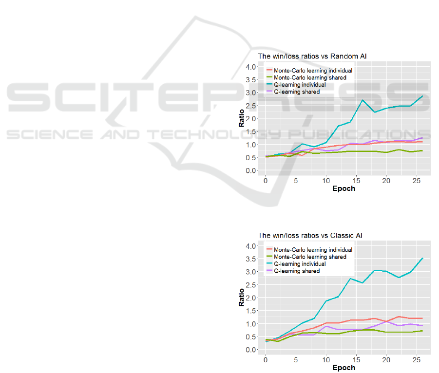
The results that were gathered are plotted in Figures

2 - 5. Figure 2 and Figure 3 contain the mean ratio

between wins and losses after X amount of epochs

(games) for different combinations of learning al-

gorithms and reward applications. Figure 2 shows

the ratios of every conﬁguration playing against the

random AI, while Figure 3 shows the ratios for ev-

ery conﬁguration playing against the classic (pre-

programmed) AI. The win-loss ratio shows how well

the neural network performs in comparison to the op-

ponent, a value of 1 represents equal performance. A

value higher than 1 such as the Q-learning individ-

ual rewards result in Figure 2 represents better perfor-

mance than the opponent, while a value lower than 1

represents worse performance than the opponent.

Figure 2: Graph that shows the ratio between wins and

losses for all conﬁgurations against the random AI.

Figure 3: Graph that shows the ratio between wins and

losses for all conﬁgurations against the classic AI.

Hierarchical Reinforcement Learning for Real-Time Strategy Games

475

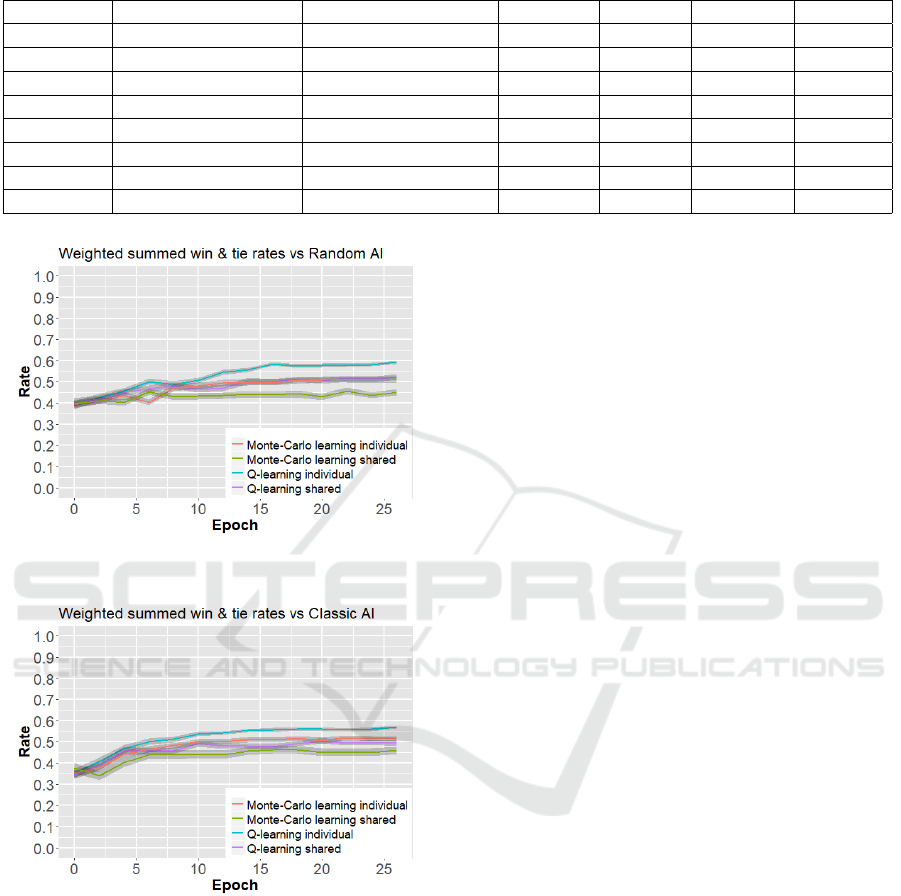
Table 3: Mean performance after 26 epochs (games).

Opponent Method Reward Application Win-rate Tie-rate Loss-rate Win:loss

Classic Q-learning Individual 19.5% 75.0% 5.5% 7:2

Classic Q-learning Shared 13.2% 72.3% 14.4% 9:10

Classic Monte Carlo method Individual 18.0% 67.0% 15.0% 6:5

Classic Monte Carlo method Shared 21.9% 48.0% 30.0% 7:10

Random Q-learning Individual 28.6% 61.5% 10.0% 3:1

Random Q-learning Shared 23.5% 57.8% 18.8% 5:4

Random Monte Carlo method Individual 28.8% 45.1% 26.2% 11:10

Random Monte Carlo method Shared 32.0% 26.2% 41.9% 3:4

Figure 4: Graph that shows the summed ratios of wins and

ties for all conﬁgurations against the random AI.

Figure 5: Graph that shows the summed ratios of wins and

ties for all conﬁgurations against the classic AI.

The results shown in Figure 4 and Figure 5 contain

the weighted sum of the mean win- and tie-rates for

all different combinations of learning algorithms and

reward applications. The win-rate has a weight of 1,

loss-rate a weight of 0 and the tie-rate has a weight of

0.5. The lines indicate the mean weighted sum while

the gray area indicates the standard deviation.

In all ﬁgures, all lines increase over time, meaning

that all conﬁgurations improve their performance dur-

ing training. One can clearly see that the combination

of Q-learning with individual rewards outperforms all

other conﬁgurations signiﬁcantly. After training, this

method achieves a ﬁnal win:loss ratio which is ap-

proximately 7:2 against the classic AI and 3:1 against

the random AI, roughly 3 times higher than the sec-

ond best conﬁguration. The weighted sum of its win-

and tie-rates are also signiﬁcantly higher than all other

combinations. It is noticeable that Q-learning out-

performs Monte Carlo learning in both performance

measures given that the other factors are equal and

individual rewards outperforms shared rewards given

the other factors are equal.

All the results measured show considerable tie-

rates. Against the classic AI the tie-rates are mostly

in the region of 65-75% and against the random AI

they are mostly between 45-65% as shown in Table

3. The exceptions for both opponents are the results

of Monte Carlo methods using a shared reward func-

tion, for which the tie-rate converges to around 50%

against the classic AI, while the tie-rate converges to

around 25% against the Random AI. This might seem

favourable, but the decrease of the tie-rate has an al-

most one to one inverse relation with the loss-rate and

is thus an overall worse result.

4.3 Discussion

The results show that individual rewards outperform

shared rewards. We suspect the reason for this that

predicting the sum of all future unit rewards is much

harder for a unit than to learn to predict its own re-

ward intake. Furthermore, Q-learning outperforms

the Monte Carlo learning method. It is known that

Monte Carlo methods have a higher variance in the

updates, which makes the learning process harder.

The encountered relatively high tie-rates that were

encountered in the measured results can be explained

as follows. A round is deemed a tie when a time-limit

of 90 seconds is reached. This feature is implemented

to reduce stagnating behaviour and allow for faster

data collection. Increasing the time limit should lower

the amount of ties.

There are several facets which deserve a closer

ICAART 2018 - 10th International Conference on Agents and Artiﬁcial Intelligence

476

look following our experiences during this research,

especially the use of different modules and the multi-

plicative effects they can have. The unit builder is a

great example. We found that having a more intelli-

gent unit builder signiﬁcantly improves performance.

Even though the unit builder is now handled by an

FSM, it implies that adding a module to the AI that

can learn which units to build would likely increase

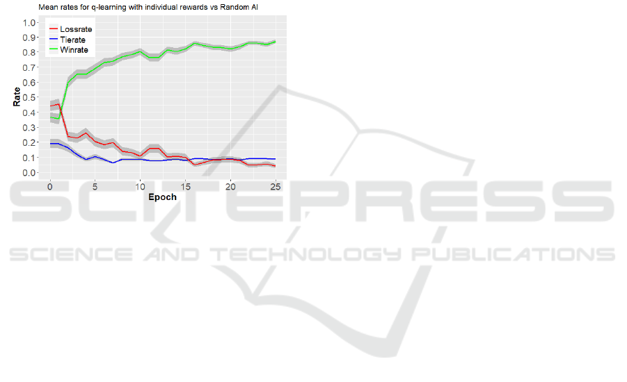
the performance as a whole signiﬁcantly. The result

of a neural network using a smart unit builder (FSM)

against our classic AI with a random unit builder can

be observed in Figure 6. One can clearly see that

the win-rate approaches 90%, which shows the im-

portance of an intelligent unit builder for this game.

Figure 6: Graph of the performance for Q-learning with

individual rewards where it has an improved unit building

algorithm compared to the opponent’s random choice.

5 CONCLUSIONS

We described several different reinforcement learning

methods for learning to play a particular RTS game.

The use of higher-order inputs and hierarchical rein-

forcement learning leads to a system which can learn

to play the game within only 26 games. The results

also show that Q-learning is better able to optimize

the team strategy than Monte Carlo methods. For as-

signing rewards to individual agents, the use of in-

dividual rewards is better than sharing the rewards

among all team members. This is most probably be-

cause predicting the intake of all shared rewards is

difﬁcult to learn for an agent given its own higher-

level game representation as input to the multi-layer

perceptron.

In future work, we would like to study the use-

fulness of more game-related input information in the

decision making process of the agents. Furthermore,

we want to use reinforcement learning techniques to

not only learn the mid-level combat strategy, but also

other tasks commonly present in an RTS game.

REFERENCES

Barto, A. and Mahadevan, S. (2003). Recent advances in

hierarchical reinforcement learning. Discrete Event

Dynamic Systems, 13:341–379.

Bom, L., Henken, R., and Wiering, M. (2013). Reinforce-

ment learning to train Ms. Pac-Man using higher-order

action-relative inputs. In Adaptive Dynamic Program-

ming and Reinforcement Learning (ADPRL), 2013

IEEE Symposium on, pages 156–163.

Buro, M. and Churchill, D. (2012). Real-time strategy game

competitions. AI Magazine, 33(3):106.

Buro, M., Lanctot, M., and Orsten, S. (2007). The second

annual real-time strategy game AI competition. Pro-

ceedings of gameon NA.

Ghory, I. (2004). Reinforcment learning in board games.

Department of Computer Science, University of Bris-

tol, Tech. Rep.

Littman, M. L. (1994). Markov games as a framework for

multi-agent reinforcement learning. In Proceedings

of the eleventh international conference on machine

learning, volume 157, pages 157–163.

Markov, A. A. (1960). The theory of algorithms. Am. Math.

Soc. Transl., 15:1–14.

Marthi, B., Russell, S. J., Latham, D., and Guestrin, C.

(2005). Concurrent hierarchical reinforcement learn-

ing. In IJCAI, pages 779–785.

Patel, P. (2009). Improving computer game bots behavior

using Q-learning. Master’s thesis, Southern Illinois

University Carbondale, San Diego.

Puterman, M. L. (1994). Markov decision processes. 1994.

John Wiley & Sons, New Jersey.

Shantia, A., Begue, E., and Wiering, M. (2011). Con-

nectionist reinforcement learning for intelligent unit

micro management in Starcraft. In Neural Networks

(IJCNN), The 2011 International Joint Conference on,

pages 1794–1801. IEEE.

Spronck, P., Ponsen, M., Sprinkhuizen-Kuyper, I., and

Postma, E. (2006). Adaptive game AI with dynamic

scripting. Machine Learning, 63(3):217–248.

Sutton, R. S. and Barto, A. G. (1998). Reinforcement learn-

ing: An introduction, volume 1. MIT press Cam-

bridge.

Szita, I. (2012). Reinforcement learning in games. In Rein-

forcement Learning State-of-the-Art, pages 539–577.

Springer.

van Seijen, H., Fatemi, M., Romoff, J., Laroche, R.,

Barnes, T., and Tsang, J. (2017). Hybrid reward ar-

chitecture for reinforcement learning. arXiv preprint

arXiv:1706.04208.

Wiering, M. and Van Otterlo, M. (2012). Reinforcement

Learning State-of-the-Art, volume 12. Springer.

Hierarchical Reinforcement Learning for Real-Time Strategy Games

477