Apoptotic Regulatory Module as Switched Control System

Analysis of Asymptotic Properties

Magdalena Ochab, Andrzej Swierniak, Jerzy Klamka and Krzysztof Puszynski

Institute of Automatic Control, Silesian University of Technology, Akademicka 16, 44-100 Gliwice, Poland

Keywords:

Biological System, Piece-wise Linear Model, Switchings.

Abstract:

Switching control systems are getting increased interests due to their capability to exhibit simultaneously

several kinds of dynamic behaviour in different parts of the system. Such hybrid systems can be applied in

many different ﬁelds. We present the application of the switched control systems in modelling a biological

system, precisely a p53-dependent apoptotic intercellular pathway. Biological experiments show that cells

exhibit variety of different behaviours for the same external stimuli. Differences in cell responses lead to

population split into fractions. We present the analysis of asymptotic properties of the apoptotic regulatory

module with respect to a parameter which describes an effect of an external stress. Results show that the

system can exhibit two types of behaviour: stabilization or oscillation near the equilibrium point.

1 INTRODUCTION

Switched control systems are a class of systems that

consist of several linear subsystems and set of switch-

ing rules among them. Such systems are character-

ized by different models in dependence on the state

of the system. As a result even simple model can

have various types of dynamic behaviour for speci-

ﬁed states of the system, which can result in chaos

or multiple limit cycles. On the other hand, switched

systems are relatively easy to analyse due to its par-

tially linear properties (Klamka et al., 2013).

Among many other applications of switched sys-

tems, they can be applied to modelling the biological

processes (Swierniak and Klamka, 2014). Biologi-

cal and biochemical reactions usually are not sponta-

neous but are regulated by variety of regulatory fac-

tors, and consequently the process rates are described

by the step-like function. To retain the switching be-

haviour majority of biological models are highly non-

linear, which implies difﬁculties in their analysis. The

piece-wise linear models are easier to create, because

values of the parameters correspond directly to the

observed processes rates. Moreover the switched sys-

tems enable analysis of the properties, which are com-

patible with biological observations. Comparison of

the nonlinear model results and the ones from piece-

wise linear model shows that the basic dynamics is

the same (Ochab et al., 2016). Switched systems can

be efﬁciently applied to modelling biological gene-

protein networks, systems with complex dynamics.

Apoptosis is intercellular process of programmed

cell death. It occurs in every multicellular organism

in damaged, defective or no longer required cells.

One of the key players in the apoptotic response to

the DNA damage is the protein p53, which activates

production of proteins responsible for apoptosis. The

proper activity of the apoptotic pathway is crucial for

the whole organism, because it enables elimination of

the damaged cells and prevents carcinogenesis (Vous-

den and Lu, 2002; Schmitt and Lowe, 1999). Huge

interest of the protein p53 and its regulatory network

among the researchers is a result of high contribution

of the cell with its p53 abnormalities in the cancer

cells.

The main activity of the p53 is regulation protein

production by acting as transcription factor. In nor-

mal healthy cell the low p53 level is maintained by

the negative coupling with MDM2. The p53 activates

MDM2 production, which in turn induces p53 degra-

dation. External stress, such as DNA damage, induces

MDM2 degradation. Decrease of the MDM2 results

in stabilization of p53 and activation of the proteins

production which are responsible for cell cycle block-

ade, damaged DNA repair and apoptosis. Results of

biological experiments show that, depending on the

stress level, the p53 can be maintained on different

levels (Kracikova et al., 2013). In case of low stress,

the normal cell division is blocked by the medium

level of the p53 and processes of DNA repair are ini-

Ochab, M., Swierniak, A., Klamka, J. and Puszy

nski, K.

Apoptotic Regulatory Module as Switched Control System - Analysis of Asymptotic Properties.

DOI: 10.5220/0006593601190126

In Proceedings of the 11th International Joint Conference on Biomedical Engineering Systems and Technologies (BIOSTEC 2018) - Volume 3: BIOINFORMATICS, pages 119-126

ISBN: 978-989-758-280-6

119

tiated. However in this state the p53 level is not high

enough to induce the process of apoptosis. Top level

of external stress activates the positive feedback loop,

which works through protein PTEN. Protein PTEN is

induced by p53, and after accumulation in cytoplasm

is able to block the negative feedback by blocking the

MDM2 transport to nucleus. As a result the p53 in-

creases to high level and apoptosis is activated (Jonak

et al., 2016). Due to the great signiﬁcance of the

p53-dependent apoptotic pathway a wide range of ex-

periments, both biological and mathematical, are per-

formed to acquire fully knowledge about this process.

In our previous research we have examined the

system behaviour for three different stress levels: 0,

4 and 9 a.u. (Ochab et al., 2017a). In present paper

we study possible system responses and thus we focus

our attention on the asymptotic properties of the con-

trol system for the whole range of parameter R, which

stands for a level of stress.

2 METHODS

2.1 PLDE Model Analysis

Piece-wise linear differential equation models (PLDE

models) consist of set of linear differential functions

and set of rules deﬁning the subset of functions, which

is used for a speciﬁed state. For biological systems the

general equation is deﬁned as:

= p

(X) − d

(X)x

, i = 1, 2,..., n (1)

where x

is a protein, p

is a production rate, d

is a

degradation rate and X is a state of the system de-

scribed by the set of boolean functions. The phase

space is divided by thresholds into regulatory do-

mains. In each domain the system is described by a

linear (afﬁne) model. The boundaries of the domains

are deﬁned by threshold values denoted by θ

i j

, where

i is the variable (protein) and j is a number of the

threshold for the given variable. On the boundaries,

values of the parameters can switch and consequently

the system is not continuous. Additionally the sys-

tem contains switching variables, which deﬁne if the

speciﬁc variable is above or below its threshold. The

switching variables are boolean and are denoted by

, where i indicates a number of the variable. The

boolean variables are applied to deﬁne the regulatory

domains. Each domain is deﬁned by a boolean vec-

tor B which speciﬁes relation of all the variables to its

threshold. Moreover relation between variables and

thresholds deﬁnes the values of the parameters in the

model.

In the piece-wise linear models two types of sta-

tionary points are distinguished: regular stationary

points and singular stationary points.

2.1.1 RSP

The regular stationary points, shortly RSPs, exist in-

side the regulatory domain. The RSPs are localized

by application of steady state condition for each do-

main. If the calculated point lies inside boundaries of

the considered domain, it is asymptotically stable and

is called RSP. A method determining RSP can be de-

scribed as follows:

for each subsystem described by linear equation

model

• calculate steady state dx

/dt = 0

• check localization of the point, if the point lies

inside the boundaries, it is the RSP.

2.1.2 SSP

Localization of the singular stationary points, shortly

SSPs, is much more challenging, because they exist

when at least one of the variables lies on its threshold.

In our analysis we use the method proposed for gene

regulatory networks (Plahte et al., 1994; Mestl et al.,

1995; Plahte et al., 1998). In the simplest case only

one variable is equal to its threshold which means that

the SSP is located on the boundary.

The SSPs can be described by a number of the

variables which lie on the threshold. In the simplest

case only one variable is located on the boundary and

the other variable values are not restricted. It is wor-

thy to notice that such case is possible only if the vari-

able is directly dependent on its own threshold value.

To be precise, the SSP lies on the threshold θ

i j

for

variable x

= θ

i j

, if the derivative ∂F

/∂Z

i j

is greater

than 0, where F

is the time derivative dx

/dt and Z

i j

is switching variable.

The switched system is not continuous on the

thresholds, so to calculate the derivatives, we replace

the step function by the continuous sigmoid function

with the limit [0,1]. Thus the switching function is a

monotonic molliﬁer deﬁned as Z

i j

= Z(x

,θ

i j

,δ):

i j











0 for x

≤ θ

i j

− δ,

increases from 0 to 1 for x

∈ hθ

i j

− δ,θ

i j

+ δi

1 for x

≥ θ

i j

+ δ

Parameter δ denotes the distance from the threshold,

so with δ tending to zero, the monotonic molliﬁer ap-

proaches the step function.

In order to determine existence of the SSP in

the case when two or more variables are equal to

BIOINFORMATICS 2018 - 9th International Conference on Bioinformatics Models, Methods and Algorithms

120

their thresholds, we apply the procedure described by

Mestl et al. (Mestl et al., 1995). For all sets of the

threshold variables:

• replace values of the variables by corresponding

thresholds

• determine values of the switching variables,

which are not related to the analysed thresholds,

as 0 or 1

• set time derivatives to 0

• solve the set of equations to calculate values of

switching variables related to the analysed thresh-

olds

• check assumptions: values of switching variables

must be included in the range [0,1] and values

of remaining variables must be in the speciﬁed

range, if yes, there is a SSP

In the system with SSP localized on the crossing

of boundaries oscillations can be observed, because

there exist a limit cycle around the SSP.

2.2 p53-Dependent Apoptotic Model

A piece-wise linear model of the p53 regulatory mod-

ule was presented in our previous paper, where we

compared its results with the results obtained by the

nonlinear model (Ochab et al., 2016). The model

consists of 4 variables, which correspond to different

types of proteins: P - p53, C - cytoplasmic MDM2,

N - nuclear MDM2, T - PTEN. Production of p53

(P) is constant and its degradation is increased by nu-

clear MDM2 (N). Production of cytoplasmic MDM2

MDM2 (N)results from nuclear import of the cyto-

plasmic form (C), which is regulated by T . Conse-

quently in this system two feedback loops exist. The

ﬁrst one is negative and it exists between P, C and

N, because p53 (P) induces production of its own in-

hibitor. The second one is positive, due to blockade of

the negative feedback by PTEN (T ), which is induced

by p53 (P). All the dependencies between proteins

are presented on the diagram (Fig. 1).

We introduce 4 threshold to divide phase space

into regulatory domains. There is one threshold value

for p53 in order to model the activation of MDM2 and

PTEN production (parameters p

∗

and p

∗

respectively)

by accumulated p53. One threshold for PTEN is used

to model the blockade of the MDM2 transport to nu-

cleus. PTEN level exceeding the threshold value sig-

niﬁes decrease of the MDM2 transport rate (k

∗

). Ad-

ditionally there are two threshold values for nuclear

MDM2, which separates the three levels of p53 degra-

dation: low, medium and high. There are no threshold

Figure 1: Model of the p53 regulatory core. Symbols of

the variables, switching variables and model parameters are

taken from the model (2).

for cytoplasmic MDM2, because none of the analysed

processes are dependent on its level. Due to existence

of four thresholds, the model contains four switching

variables Z

, Z

, which deﬁne if the spe-

ciﬁc variable is above or below its threshold. More-

over each domain is deﬁned by a vector B = [P,N, T ],

where P, N and T are the boolean-like states denoting

if the corresponding variable is below (0) or above (1

in case of P and T and 1 or 2 in case of N) its thresh-

old. For example domain [110] denotes the subspace,

where P > θ

, θ

< N < θ

and T < θ

. Please,

note that parameters which are dependent on the sys-

tem state are marked with

∗

The control system is linear, precisely afﬁne, with

a constant input. The general linear differential state

equation can be written in the following form:

x(t) = Ax(t) + b, t ∈ [0, +∞) (2)

where the x(t) ∈ R

is a state vector, A is a given n ×n

- dimensional control matrix and b ∈ R

is a constant

input. They are deﬁned below:

x(t) =







P(t)

C(t)

N(t)

T (t)







b =







∗







Moreover,

A =







−d

∗

0 0 0

0 −(k

∗

+ d

(1 + R)) 0 0

0 k

∗

−d

(1 + R) 0

0 0 0 −d







where

∗

= p

+ p

∗

= p

+ p

∗

= d

+ d

∗

= k

− k

Apoptotic Regulatory Module as Switched Control System - Analysis of Asymptotic Properties

121



0 if P < θ

1 if P > θ



0 if N < θ

1 if N > θ



0 if N < θ

1 if N > θ



0 if T < θ

1 if T > θ

The degradation of the MDM2, both cytoplasmic

and nuclear, is increased by stress factor denoted by

R. The values of the parameters given above are pre-

sented in Table 1 and the values of threshold are pre-

sented in Table 2 Values of the parameters base on our

previous research (Ochab et al., 2016) and the biolog-

ical results (Jonak et al., 2016).

3 RESULTS

As we showed in our previous paper (Ochab et al.,

2017a), for different size of stress - reﬂected by dif-

ferent values of the parameter R, the system response

can be signiﬁcantly different. In order to check all

possible realizations of the system for whole range

of stress, we examine existence of the different RSPs

and SSPs for R ∈ [0, +∞i. The system behaviour for

speciﬁed values of R can be visualized by the transi-

tion diagram. The domains are marked by the rect-

angles with vectors determining their states. The ar-

rows show the directions of the transitions between

domains. Transition diagrams show in which domain

the RSPs exist and are useful in localizing the closed

sequences between domains, which can contain the

SSPs around which the systems response can oscil-

late. The simplest way to create transition diagram is

calculation of the RSP in each domain and determine

whether the solution stay in the analysed domain or

move to another. Exemplary, for stress R = 5, there is

one RSP in the system in the domain [101] and one

possible limit cycle between domains [010], [110],

[120] and [020] (Fig. 2).

3.1 Regular Stationary Point - RSP

In this section we determine ranges of the R in which

the RSP exists in any domain. For each domain we

write the model equations and equal them to 0. Then

we solve the system of equation to ﬁnd values of

R, which assures that the stationary point lays inside

analysed domain. In the apoptotic switched model the

Figure 2: State transition diagram for the apoptotic model

for R = 5. Gray domain contains RSP, bold arrows empha-

size the closed sequence around the SSP.

regular stationary points can exist only in 3 domains.

The RSPs exist:

• in domain [020] for R ∈ [0,0.8635i

• in domain [111] for R ∈ h1.0322,1.9154i

• in domain [101] for R ∈ h1.9154,+∞i.

The values of the variable P in the steady states

in each domain are presented in table 3. For R ∈

[0.8635,1.0322i there is no RSP in the system, so the

system response does not stabilize on one value but

oscillates in a limit cycle.

The regular stationary points correspond to the

asymptotically stable cell response in different cases.

For low stress the RSP exists in domain [020] and cor-

responds to the low p53 level and the high nuclear

MDM2 level, which agrees with biological observa-

tion of normal cells, where low p53 level is main-

tained by high degradation rate and, in turn by high

MDM2 level. An increase of the parameter R results

in disappearing of the RSP in domain [020] and aris-

ing in domain [111] and afterwards in [101]. The in-

crease of the R corresponds to higher external stress

level, which induces cell damages, the MDM2 degra-

dation and consequently accumulation of the p53 (see

Table 3 with increasing values of p53 in stationary

points).

In biological experiments after high stress level

the increased p53 level is observed. The p53 level in

cell determines the cell response, the medium average

p53 level can be assigned to the cells with repairable

damages and excluded proliferation, whereas the high

p53 level indicates cells with unrepairable damages

and apoptosis activation.

3.2 Singular Stationary Point - SSP

In the apoptotic model thresholds exist for 3 vari-

ables: P, N and T, and consequently, the SSP can

exist in 3 types of subspaces: on the plane where one

BIOINFORMATICS 2018 - 9th International Conference on Bioinformatics Models, Methods and Algorithms

122

Table 1: The values of the model parameters.

Parameter Description Value Unit

spontaneous P production rate 8.8 1/sec

spontaneous C production rate 2.4 1/sec

P-induced C production rate 21.6 1/sec

spontaneous T production rate 0.5172 1/sec

P-induced T production rate 3.6204 1/sec

spontaneous P degradation rate 9.8395 ∗ 10

−5

1/sec

N-induced P degradation rate 6.5435 ∗ 10

−5

1/sec

N-induced P degradation rate 1.6283 ∗ 10

−4

1/sec

spontaneous C and N degradation rate 1.375 ∗ 10

−5

1/sec

spontaneous T degradation rate 3 ∗ 10

−5

1/sec

spontaneous N transport rate 1.5 ∗ 10

−4

1/sec

T -inhibited N transport rate 1.4713 ∗ 10

−4

1/sec

Table 2: The values of the thresholds for variables.

Thresholds Description Value Unit

P threshold value 4.5 ∗ 10

molecules

N threshold value 4 ∗ 10

molecules

N threshold value 8 ∗ 10

molecules

T threshold value 1 ∗ 10

molecules

Table 3: Values of p53 (P) in regular stationary point for

different values of stress R.

R Domain P

0 - 0.8635 [020] 3.3559 ·10

1.0322 - 1.9154 [111] 5.3714 · 10

1.9154 - +∞ [101] 8.9435 ·10

variable lies on its threshold, on the crossing of the

planes, where two variables lie on thresholds, and on

the point, where all three variables lie on their thresh-

olds.

In order to check if the model can contain the

SSP on the plane, we calculate the derivatives of all

the variables with respect to its switching variables

∂F

/∂Z

i j

. In this model partial derivatives for all the

variables P, C, N and T do not directly depend on

their switching variables Z

i j

so all ∂F

/∂Z

i j

are equal

to zero. Consequently in this system there is no SSP

on the surface of the single boundary.

To determine an existence of the SSP on the cross-

ing of two boundaries we analyse all the existed cases.

For all combinations of two thresholds from θ

, θ

and θ

or θ

the procedure described in section

2.1.2 was applied with attitude to determine values of

the stress R, for which the assumptions are satisﬁed.

For the whole range of the parameter R, the SSP can

exist only in two subspaces.

3.2.1 SSP 1: [θ

, θ

, T < θ

]

The SSP exists on the crossing of the threshold of the

p53 and the MDM2, precisely for P equal to θ

, N

equal to θ

and T smaller than θ

. The model equa-

tions describing the steady state in this subspace are

as follows:

0 = p

− (d

+ d

)θ

0 = p

+ p

− (k

+ d

(1 + R))C ,

0 = k

C − d

(1 + R)θ

0 = p

+ p

− d

T. (3)

The switching parameters Z

and Z

are in the

range [0,1] and the value of the T variable is smaller

than θ

for R ∈ h0.8635, 7.7038i.

3.2.2 SSP 2: [θ

, θ

, T > θ

]

The second SSP in the system exists for P equal to

, N equal to θ

and T greater than θ

. The model

equations describing the steady state are presented be-

low:

0 = p

− (d

+ d

)θ

0 = p

+ p

− (k

− k

+ d

(1 + R))C ,

0 = (k

− k

)C − d

(1 + R)θ

0 = p

+ p

− d

T. (4)

Apoptotic Regulatory Module as Switched Control System - Analysis of Asymptotic Properties

123

The switching parameters Z

and Z

are in the

range [0, 1] and the value of the T variable is greater

than θ

for R ∈ h0.7059, 1.0322i.

The last possible case, is localization of the SSP

in the crossing of three boundaries. In this model two

such points exist and should be analyzed: [θ

, θ

] and [θ

, θ

]. In both cases the values of the

switching variables Z

, Z

(or Z

) and Z

are not

included in the range [0,1] so independently of the

parameter R, the SSP cannot exist there.

Due to an existence of the SSPs in two subspaces,

two types of oscillations can be observed. Signiﬁ-

cantly wider range of the parameter R have the SSP

in the region [θ

, θ

, T < θ

]. This SSP results

in undamped oscillations between low and high p53

level and medium and high MDM2 level. Such os-

cillations are a consequence of the negative feedback

loop, and are related to the delayed cell response in

case of the repairable damages. Biological experi-

ments show that for the low stress level a cell makes

an attempt to repair its damages and comes back to the

normal state. The oscillation of the p53 level prevents

cell division but in the same time does not induce

cell elimination (Geva-Zatorsky et al., 2006; Bar-Or

et al., 2000). Consequently if the damages are not un-

repairable, the cell has got time to come back to the

normal state.

The second SSP indicates an existence of the cy-

cle between the p53 and the MDM2 for high PTEN

level. Such situation occurs only for a very narrow

range of R parameters. This case is possible for low

external stress, when the initial high PTEN level is

maintained over the θ

threshold by oscillation be-

tween low and high p53 level. However in biological

cells high PTEN level is observed only after p53 ac-

tivation, so such situation is not probable concluding

from the biological results.

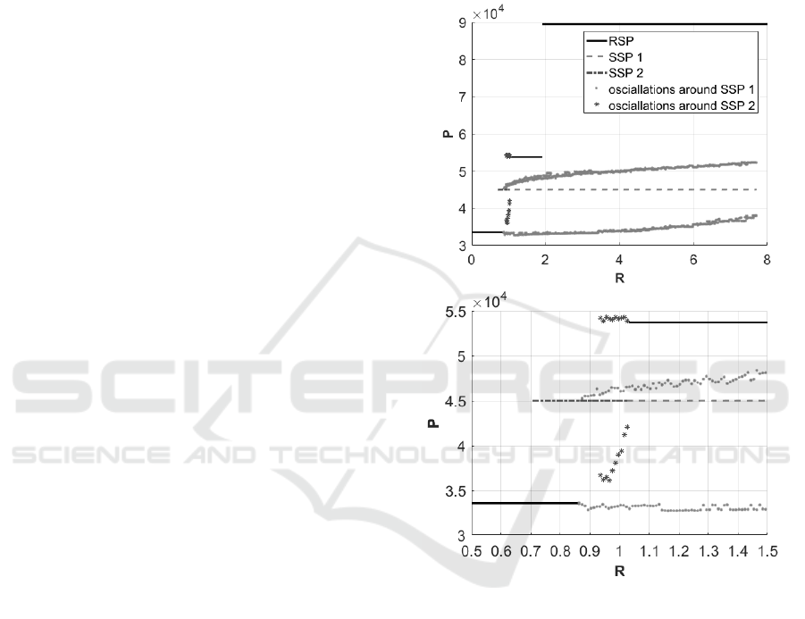
3.3 Bifurcation Diagram

Depending on the R parameter value, the stationary

points exist in different domains or on the different

boundaries. For small R the RSP exists in domain

[020] and the P level is low. With increase of the R

value, in the system the second stationary point, SSP,

appears. Depending on the initial conditions the sys-

tem can stabilize in the domain [020] or oscillate be-

tween domains with low and high P and medium and

high N. With further increase of the R, in the system

any RSP does not exist, so the only possible system

response is oscillation. In quite narrow range of the R

parameter values, in the system two singular station-

ary points exist, which results in two different cycles

and different levels of proteins. With further increase

of R, in the system the RSP in the domain [111] arises,

which is characterized by the medium P level. For R

greater than 1.9154 in the system the RSP arises in the

domain [101] with the high P level. The SSP exists in

the system for R smaller than 7.7038 which means,

that depending on the initial conditions, in the system

two types of response can be observed: stabilization

or oscillations (see Fig. 3).

Figure 3: Level of the variable P in dependency on the pa-

rameter R. Top ﬁgure: results for the whole range of R.

Bottom ﬁgure: magniﬁcation of the ﬁgure for R = h0.51.3i.

SSP 1 - values of P in the SSP with T < θ

, SSP 2 - values

of P in the SSP with T > θ

. Please notice the lack of os-

cillations around SSP 2 for R ∈ h0.8635, 0.95i - see text for

explanation.

The dependency between variables N and R is pre-

sented on the Fig. 4. With increase of R, the N level is

decreased. For a wide range of the R parameter, in the

system two types of result exists, stabilization in the

steady state or oscillation of the protein levels, which

are a consequence of the simultaneous existence of

the two stationary points: SSP and RSP.

Notice the lack of oscillations around SSP for R ∈

h0.8635,0.95i on Fig. 3 (bottom panel). It is caused

by the close proximity of the SSP to the θ

bound-

ary which causes that the trajectories escape from the

BIOINFORMATICS 2018 - 9th International Conference on Bioinformatics Models, Methods and Algorithms

124

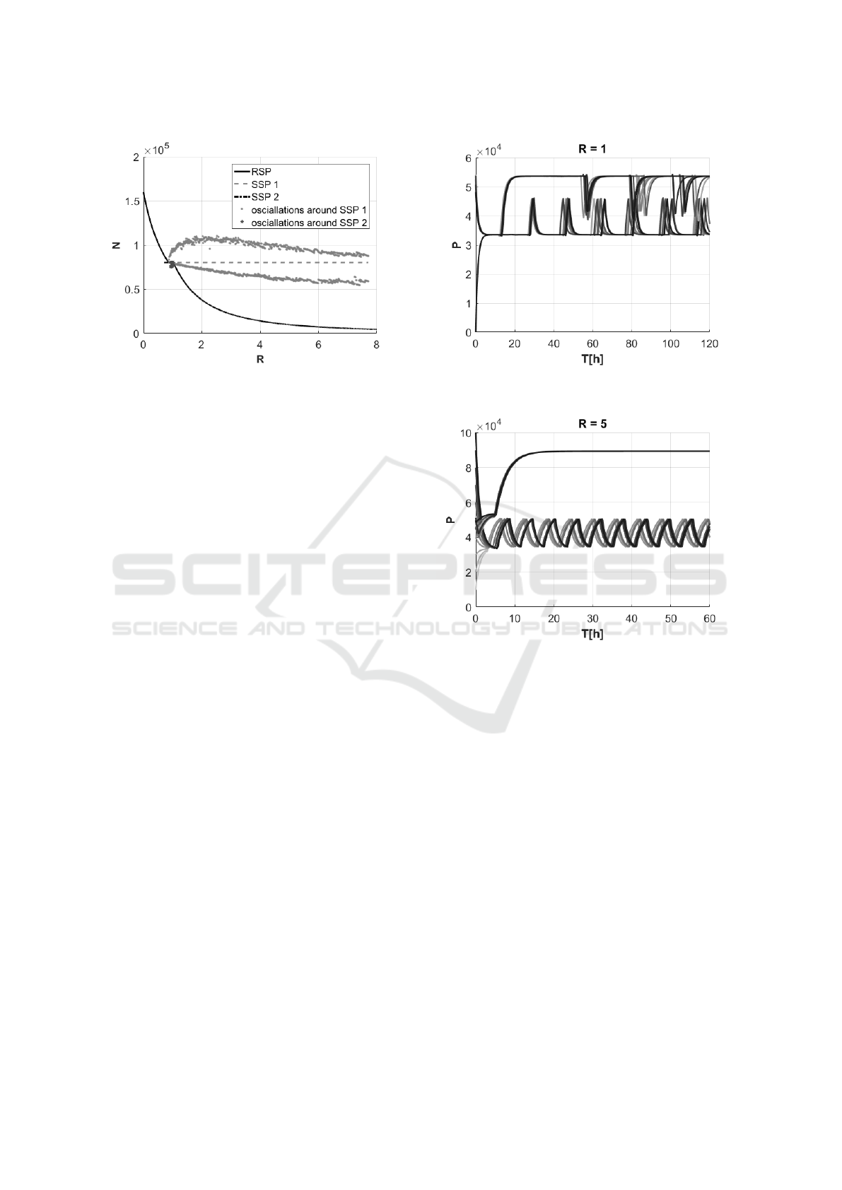
Figure 4: Level of the variable N in dependency on the pa-

rameter R. SSP 1 - values of N in the SSP with T < θ

, SSP

2 - values of N in the SSP with T > θ

oscillatory mode. With the increasing R, SSP recedes

from the θ

boundary and with R greater than 0.95,

trajectories do not cross the threshold θ

thus oscil-

lations appear. Nevertheless the presented method is

unable to detect analytically this phenomenon which

is its weakness.

More generally the weakness of the presented

method is impossibility to analytically determine the

attraction pools for the calculated stationary points.

The numerical simulation for different initial condi-

tions shows, that in the case of [θ

, θ

, T > θ

] the

attraction pool is very small.

3.4 Numerical Results

To testify the achieved results we calculated the sys-

tem response for two values of parameter R for differ-

ent initial conditions. For R equals 1, in the system

two SSPs exist and consequently on the time courses

the two types of oscillations are observed. Interest-

ingly both SSPs are on the same borders, precisely

for subspaces with P = θ

and N = θ

, but one point

is under θ

threshold and the second one is above.

Consequently, even if the values of the variable P in

the stationary points are the same, the time courses are

signiﬁcantly different (Fig. 5). For the higher value of

R, in the system one RSP and one SSP exist. Conse-

quently, depending on the initial conditions, the sys-

tem can approach the steady point in the domain [101]

or oscillate in the limit cycle around the singular sta-

tionary point (Fig. 6). In the case of modelling cell

population using stochastic approach, different types

of responses are received. Consequently the cell pop-

ulation is divided into several fractions, which present

different behaviours (Ochab et al., 2017b).

Figure 5: Time course of the variable P for different initial

conditions for value of parameter R equals 1.

Figure 6: Time course of the variable P for different initial

conditions for value of parameter R equals 5.

4 CONCLUSIONS

Analysis of the switched system demonstrate the

properties of the apoptotic intercellular pathway. The

localization and the types of the existing stationary

points correspond with the biological results. The

presented method can be efﬁciently applied to piece-

wise linear systems to examine properties of the

protein regulatory networks, nevertheless the results

show that this method is not free from imperfections.

Lack of the analysis of the attraction pools can lead to

false determination of the system behaviour based on

existence of the singular stationary points without at-

traction pools. In the future we want to overcome this

difﬁculty and improve the proposed methodology.

Apoptotic Regulatory Module as Switched Control System - Analysis of Asymptotic Properties

125

ACKNOWLEDGEMENT

The research presented here was partially supported

by the National Science Centre in Poland granted

with decision number DEC-2016/23/B/ST6/03455

(for KP), DEC-2014/13/B/ST7/00755 (for AS and

JK) and BKM- 508 /RAU1/2017 t. 6 (MO).

Calculations were performed on the Ziemowit

computational cluster created in the EU Innovative

Economy Operational Programme (POIG).02.01.00-

00-166/08 project (BIO-FARMA) and expanded in

the POIG.02.03.01-00-040/13 project (Syscancer)

(http://www.ziemowit.hpc.polsl.pl).

REFERENCES

Bar-Or, R. L., Maya, R., Segel, L. A., Alon, U., Levine,

A. J., and Oren, M. (2000). Generation of oscilla-

tions by the p53-mdm2 feedback loop: a theoretical

and experimental study. Proceedings of the National

Academy of Sciences, 97(21):11250–11255.

Geva-Zatorsky, N., Rosenfeld, N., Itzkovitz, S., Milo, R.,

Sigal, A., Dekel, E., Yarnitzky, T., Liron, Y., Polak, P.,

Lahav, G., et al. (2006). Oscillations and variability in

the p53 system. Molecular systems biology, 2(1).

Jonak, K., Kurpas, M., Szoltysek, K., Janus, P., Abramow-

icz, A., and Puszynski, K. (2016). A novel mathemat-

ical model of atm/p53/nf-κ b pathways points to the

importance of the ddr switch-off mechanisms. BMC

systems biology, 10(1):75.

Klamka, J., Czornik, A., and Niezabitowski, M. (2013).

Stability and controllability of switched systems. Bull.

Pol. Acad. Sci., Tech. Sci. (Online), 61(3):547–555.

Kracikova, M., Akiri, G., George, A., Sachidanandam, R.,

and Aaronson, S. (2013). A threshold mechanism me-

diates p53 cell fate decision beteen growth arrest and

apoptosis. Cell Death Differ, 20:576–588.

Mestl, T., Plahte, E., and Omholt, S. W. (1995). A mathe-

matical framework for describing and analysing gene

regulatory networks. Journal of Theoretical Biology,

176(2):291–300.

Ochab, M., Puszynski, K., and Swierniak, A. (2016). Appli-

cation of the piece-wise linear models for description

of nonlinear biological systems based on p53 regula-

tory unit. In Proc. XXI National Conference on Ap-

plications of Mathematics in Biology and Medicine,

Sandomierz, pages 85–90.

Ochab, M., Puszynski, K., Swierniak, A., and Klamka, J.

(2017a). Variety behavior in the piece-wise linear

model of the p53-regulatory module. In International

Conference on Bioinformatics and Biomedical Engi-

neering, pages 208–219. Springer.

Ochab, M., Swierniak, A., Klamka, J., and Puszynski, K.

(2017b). Inﬂuence of the stochasticity in threshold

localization on cell fate in the plde-model of the p53

module. In Polish Conference on Biocybernetics and

Biomedical Engineering, pages 205–217. Springer.

Plahte, E., Mestl, T., and Omholt, S. W. (1994). Global

analysis of steady points for systems of differential

equations with sigmoid interactions. Dynamics and

Stability of Systems, 9(4):275–291.

Plahte, E., Mestl, T., and Omholt, S. W. (1998). A method-

ological basis for description and analysis of systems

with complex switch-like interactions. Journal of

mathematical biology, 36(4):321–348.

Schmitt, C. A. and Lowe, S. W. (1999). Apoptosis and ther-

apy. J. Pathol, 187:127–137.

Swierniak, A. and Klamka, J. (2014). Comparison of con-

trollability conditions for models of antiangiogenic

and combined anticancer therapy. In Proc. 19th World

Congress The International Federation of Automatic

Control, Cape Town.

Vousden, K. H. and Lu, X. (2002). Live or let die: the cell’s

response to p53. Nature, 2:594–604.

BIOINFORMATICS 2018 - 9th International Conference on Bioinformatics Models, Methods and Algorithms

126