Area Protection in Adversarial Path-finding Scenarios with Multiple
Mobile Agents on Graphs
A Theoretical and Experimental Study of Strategies for Defense Coordination
Marika Ivanov
´
a
1
, Pavel Surynek
2
and Katsutoshi Hirayama
3
1
Department of Informatics, University of Bergen, Thormhlensgt. 55, 5020 Bergen, Norway
2
National Institute of Advanced Industrial Science and Technology (AIST), 2-3-26, Aomi, Koto-ku, Tokyo 135-0064, Japan
3
Kobe University, 5-1-1, Fukaeminami-machi, Higashinada-ku, Kobe 658-0022, Japan
Keywords:
Graph-based Path-finding, Area Protection, Area Invasion, Asymmetric Goals, Mobile Agents, Agent
Navigation, Defensive Strategies, Adversarial Planning.
Abstract:
We address a problem of area protection in graph-based scenarios with multiple agents. The problem consists
of two adversarial teams of agents that move in an undirected graph. Agents are placed in vertices of the graph
and they can move into adjacent vertices in a conflict-free way in an indented environment. The aim of one
team - attackers - is to invade into a given area while the aim of the opponent team - defenders - is to protect
the area from being entered by attackers. We study strategies for assigning vertices to be occupied by the team
of defenders in order to block attacking agents. We show that the decision version of the problem of area
protection is PSPACE-hard. Further, we develop various on-line vertex-allocation strategies for the defender
team and evaluate their performance in multiple benchmarks. Our most advanced method tries to capture
bottlenecks in the graph that are frequently used by the attackers during their movement. The performed
experimental evaluation suggests that this method often defends the area successfully even in instances where
the attackers significantly outnumber the defenders.
1 INTRODUCTION
We address an Area Protection Problem (APP) with
multiple mobile agents moving in a conflict-free way.
APP can be regarded as a modification of known
problem of Adversarial Cooperative Path Finding
(ACPF) (Ivanov
´
a and Surynek, 2014) where two
teams of agents compete in reaching their target po-
sitions. Unlike ACPF, where the goals of teams of
agents are symmetric, the adversarial teams in APP
have different objectives. The first team of attackers
consists of agents whose goal is to reach a pre-defined
target location in the area being protected by the sec-
ond team of defenders. Each attacker has a unique
target in the protected area. The opponent team of
defenders tries to prevent the attackers from reaching
their targets by occupying selected locations so that
they cannot be passed by attackers.
Another distinction between ACPF and APP is a
definition of victory of a team. A team in ACPF wins
if all its agents reach their targets and agents of no
other team manage to do so earlier. In APP, the team
of defenders wins if all attackers are kept out of their
targets. Our effort is to design a strategy for the de-
fending team, so the success is measured from the de-
fenders’ perspective. It is often not possible to pre-
vent all attackers from reaching their targets, and so
the following objective functions can be pursued:
1. maximize the number of target locations that are
not captured by the corresponding attacker
2. maximize the number of target locations that are
not captured by the corresponding attacker within
a given time limit
3. maximize the sum of distances between the at-
tackers and their corresponding targets
4. minimize the time spent at captured targets
The common feature of APP and ACPF is that
once a location is occupied by an agent, it cannot be
entered by another agent until it is first vacated by the
agent which occupies it (opposing agent cannot push
the agent out). This is utilized both in competition for
reaching goals in ACPF, where agents may try to slow
down the opponent by occupying certain locations, as
184
Ivanová, M., Surynek, P. and Hirayama, K.
Area Protection in Adversarial Path-finding Scenarios with Multiple Mobile Agents on Graphs - A Theoretical and Experimental Study of Strategies for Defense Coordination.
DOI: 10.5220/0006583601840191
In Proceedings of the 10th International Conference on Agents and Artificial Intelligence (ICAART 2018) - Volume 1, pages 184-191
ISBN: 978-989-758-275-2
Copyright © 2018 by SCITEPRESS – Science and Technology Publications, Lda. All rights reserved

well as in APP, where it is a key tool for the defenders
for keeping attackers out of the protected area.
APP has many real-life motivations from the do-
mains of access denial operations both in civil and
military sector, robotics with adversarial teams of
robots or other type of penetrators (Agmon et al.,
2011), and computer games.
Our contribution consists in analysis of computa-
tional complexity of APP. In particular, we show that
APP is PSPACE-hard. Next, we suggest several on-
line solving algorithms for the defender team that al-
locate selected vertices to be occupied so that attacker
agents cannot pass into the protected area. We iden-
tify suitable vertex allocation strategies for diverse
types of APP instances and test them thoroughly.
1.1 Related Work
Movements of agents at low reactive level are as-
sumed to be planned by some cooperative path-
finding - CPF (multi-agent path-finding - MAPF) (Sil-
ver, 2005; Ryan, 2008; Wang and Botea, 2011) algo-
rithm where agents of own team cooperate while op-
posing agents are considered as obstacles. In CPF the
task is to plan movement of agents so that each agent
reaches its unique target in a conflict free manner.
There exist multiple CPF algorithms both com-
plete and incomplete as well as optimal and sub-
optimal under various objective functions.
A good trade-off between the quality of solutions
and the speed of solving is represented by subopti-
mal/incomplete search based methods which are de-
rived from the standard A* algorithm. These meth-
ods include LRA*, CA*, HCA*, and WHCA* (Silver,
2005). They provide solutions where individual paths
of agents tend to be close to respective shortest paths
connecting agents’ locations and their targets. Con-
flict avoidance among agents is implemented via a so
called reservation table in case of CA*, HCA*, and
WHCA* while LRA* relies on replanning whenever a
conflict occurs. Since our setting in APP is inherently
suitable for a replanning, the algorithm LRA* is a can-
didate for underlying CPF algorithm for APP. More-
over, LRA* is scalable for large number of agents.
Aside from CPF algorithms, systems with mobile
agents that act in the adversarial manner represent an-
other related area. These studies often focus on pa-
trolling strategies that are robust with respect to var-
ious attackers trying to penetrate through the patrol
path (Elmaliach et al., 2009).
Theoretical or empirical works related to APP also
include studies on pursuit evasion (Hespanha et al.,
1999; Vidal et al., 2002) or predator-prey (Benda
et al., 1986; Haynes and Sen, 1995) problems. The
Tileworld (Pollack and Ringuette, 1990) also provides
an experimental environment to evaluate planning and
scheduling algorithms for a team of agents. A ma-
jor difference between these works and the concept of
APP is that, unlike the previous works, we assume the
agents in each team perform CPF algorithms, which
provide a new foundation of team architecture.
1.2 Preliminaries
The environment is modeled by an undirected un-
weighted graph G = (V,E). We restrict the instances
to 4-connected grid graphs with possible obstacles.
The team of attackers and defenders is denoted by
A = {a
1
,...,a
m
} and D = {d
1
,...d
n
}, respectively.
Continuous time is divided into discrete time steps.
Agents are placed in vertices of the graph at each
time step so that at most one agent is placed in each
vertex. Let α
t
: A ∪ D → V be a uniquely invertible
mapping denoting configuration of agents at time step
t. Agents can wait or move instantaneously into ad-
jacent vertex between successive time steps to form
the next configuration α
t+1
. Abiding by the follow-
ing movement rules ensures preventing conflicts:
• An agent can move to an adjacent vertex only if
the vertex is empty, or is being left at the same
time step by another agent
• A pair of agents cannot swap along a shared edge
• No two agents enter the same adjacent vertex at
the same time
We do not assume any specific order in which
agents perform their conflict free actions at each time
step. Our experimental implementation moves all at-
tackers prior to moving all defenders at each time
step. The mapping δ
A
: A → V assigns a unique target
to each attacker. The task in APP is to find a strat-
egy of movement for defender agents so that the area
specified by δ
A
is protected.
We state APP as a decision problem as follows:
Definition 1. The decision APP problem: Given an
instance Σ = (G,A,D,α
0
,δ
A
) of APP, is there a strat-
egy of movement for the team D of defenders, so that
agents from the team A of attackers are prevented
from reaching their targets defined by δ
A
.
In many instances it is not possible to protect all
targets. We are therefore also interested in the opti-
mization variant of the APP problem:
Definition 2. The optimization APP problem: Given
an instance Σ = (G,A,D,α
0
,δ
A
) of APP, the task is to
find a strategy of movement for the team D of defend-
ers such that the number of attackers in A that reach
their target defined by δ
A
is minimized.
Area Protection in Adversarial Path-finding Scenarios with Multiple Mobile Agents on Graphs - A Theoretical and Experimental Study of
Strategies for Defense Coordination
185

2 THEORETICAL PROPERTIES
APP is a computationally challenging problem as
shown in the following analysis. In order to study
theoretical complexity of APP, we need to consider
the decision variant of APP. Many game-like prob-
lems are PSPACE-hard, and APP is not an exception.
We reduce the known problem of checking validity of
Quantified Boolean Formula (QBF) to it.
The technique of reduction of QBF to APP is in-
spired by a similar reduction of QBF to ACPF, from
which we borrow several technical steps and lemmas
(Ivanov
´
a and Surynek, 2014). We describe the reduc-
tion from QBF using the following example. Con-
sider a QBF formula in prenex normal form
ϕ = ∃x∀a∃y∀b∃z∀c
(b ∨ c ∨ x) ∧ (¬a ∨ ¬b ∨ y)∧
(a ∨ ¬x ∨ z) ∧ (¬c ∨ ¬y ∨ ¬z) (1)
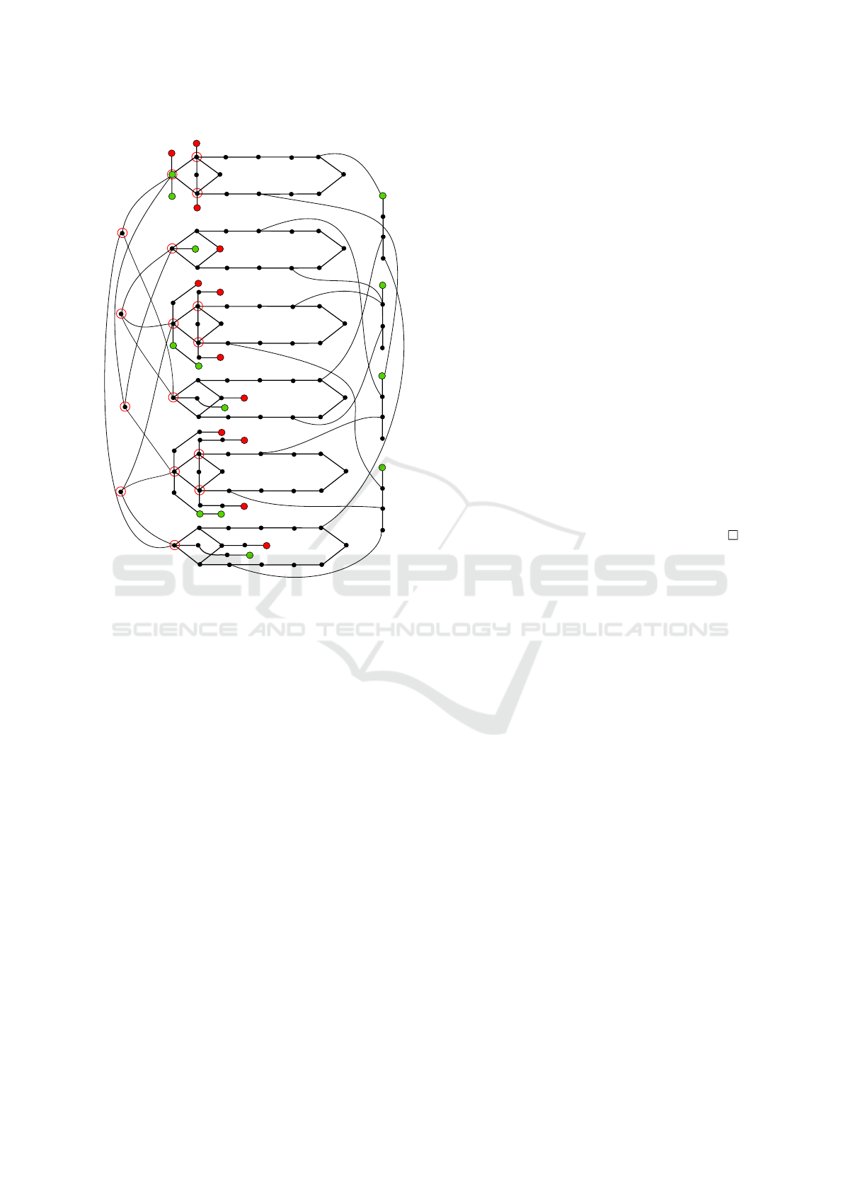
This formula is reduced to the APP instance depicted
in Fig. 4. Let n and m be the number of variables and
clauses, respectively. The construction contains three
types of graph gadgets.
For an existentially quantified variable x we con-
struct a diamond-shape gadget consisting of two par-
allel paths of length m+2 joining at its two endpoints.
t
x
1
t
2
x
t
x
m-1
t
x
m
f
x
1
f
2
x
f
x
m-1
f
x
m
a
x2
a
x1
a
x3
δ(a
x1
)
d
x1
d
x2
δ(a
x2
)
δ(a
x3
)
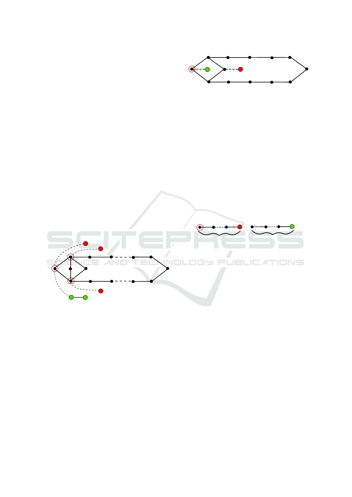
Figure 1: An existentially quantified variable gadget.
There are 4 paths connected to the diamond at spe-
cific vertices as depicted in Fig. 1. The gadget further
contains three attackers and two defenders with initial
positions at the endpoints of the four joining paths.
The vertices in red circles are targets of specified at-
tackers. The only chance for defenders d
x1
and d
x2
to
prevent attackers a
x3
and a
x1
from reaching their tar-
gets is to advance towards the diamond and occupy
δ
A
(a
x3
) by d
x2
and either δ
A
(a
x1
) or δ
A
(a
x2
) by d
x1
.
For every universally quantified variable a there
is a similar gadget with a defender d
a1
and an attacker
a
a1
whose target δ
A
(a
a1
) lies at the leftmost vertex of
the diamond structure (see Fig. 2). The defender has
to rush to the attacker’s target and occupy it, because
otherwise the target would be captured by the attacker.
Moreover, there is a gadget in two parts for each
clause C depicted in Fig. 3. It contains a simple path
t
a
1
t
2
a
t
a
m-1
t
a
m
f
a
1
f
a
m-1
f
a
m
d
a1
a
a1
δ(a
a1
)
f
a
2
Figure 2: A universally quantified variable gadget.
p of length bn/2c+1 with a defender d
C
placed at one
endpoint. The length of p is chosen in order to ensure
a correct time of d
C
’s entering to a variable gadget, so
that gradual assignment of truth values is simulated.
E.g., if a variable occurring in C stands in the second
∀∃ pair of variables in the prefix (the first and last pair
is incomplete), then p is connected to the correspond-
ing variable gadget at its second vertex. The second
part of the clause is a path of length k, with one end-
point occupied by attacker a
C
whose target δ
A
(a
C
) is
located at the other endpoint. The length k is selected
in a way that the target δ
A
(a
C
) can be protected if the
defender d
C
arrives there on time, which can happen
only if it uses the shortest path to this target. If d
C
is
delayed by even one step, the attacker a
C
can capture
its target. These two parts of the clause gadget are
connected through variable gadgets.
d
C
n/2+1
k
a
C
δ(a
C
)
Figure 3: A clause gadget.
The connection by edges and paths between vari-
able and clause gadgets is designed in a way that
allows the agents to synchronously enter one of the
paths of the relevant variable gadget. A gradual evalu-
ation of variables according to their order in the prefix
corresponds to the alternating movement of agents. A
defender d
C
from clause C moves along the path of
its gadget, and every time it has the opportunity to en-
ter some variable gadget, the corresponding variable
is already evaluated.
If there is a literal in ϕ that occurs in multiple
clauses, setting its value to true causes satisfaction of
all the clauses containing it. This is indicated by a si-
multaneous entering of affected agents to the relevant
path. Each clause defender d
C
has its own vertex in
each gadget of a variable present in C, at which d
C
can
enter the gadget. This allows a collision-free entering
of multiple defenders into one path of the gadget.
Theorem 1. The decision problem whether there ex-
ists a winning strategy for the team of defenders,
i.e. whether it is possible to prevent all attackers
from reaching their targets in a given APP instance
is PSPACE-hard.
Proof. Suppose ϕ to be valid. To better understand
validity of ϕ we can intuitively ensure that variables
ICAART 2018 - 10th International Conference on Agents and Artificial Intelligence
186

a
x2
a
x1
a
x3
d
x1
d
x2
a
y2
a
y1
a
y3
d
y1
d
y2
a
z2
d
z1
d
z2
a
z1
a
z3
a
a1
d
a1
d
b1
a
b1
a
c1
d
c1
d
C1
d
C2
d
C3
d
C4
9
7
5
4
1
2
2
6
3
2
1
1
δ(a
x3
)
δ(a
x1
)
δ(a
x2
)
δ(a
y3
)
δ(a
y1
)
δ(a
y2
)
δ(a
z3
)
δ(a
z1
)
δ(a
z2
)
δ(a
a1
)
δ(a
b1
)
δ(a
c1
)
δ(a
C1
)
δ(a
C2
)
δ(a
C3
)
δ(a
C4
)
x
a
y
b
z
c
Figure 4: A reduction from TQBF to APP. Black points rep-
resent unoccupied vertices. If two points are connected by
a line without any label, it means there is an edge between
them. A line with a label k indicates that the two points
are connected by a path of k internal vertices. Initial posi-
tions of attackers and defenders are represented by red and
green nodes, respectively. A red circle around a node means
that the node is a target of some attacker. For simplicity we
do not fully display the second part of the clause gadget.
Instead, there is a red number near the target of a clause
gadget that indicates the distance of the attacker aiming to
that target. A vertex with an agent is labeled by the agent’s
name. Labels of targets specify the associated agents.
are assigned gradually according to their order in the
prefix. For every choice of value of the next ∀-
variable there exists a choice of value for the corre-
sponding ∃-variable so that eventually the last assign-
ment finishes a satisfying valuation of ϕ. The strategy
of assigning ∃ variables can be mapped to a winning
strategy for defenders in the APP instance constructed
from ϕ. Every satisfying valuation guides the defend-
ers towards vertices resulting in a position where all
targets are defended. Every time a variable is valu-
ated, another agent in the constructed APP instance is
ready to enter the upper path, if the variable is eval-
uated as true, or the lower path, otherwise. Note that
the vertices on the paths are labeled as t and f in-
dicating the truth value that is simulated by passing
through a path. When the evaluated variable x is exis-
tentially quantified, the defender d
x1
enters the upper
or lower path. In case of universally quantified vari-
able a, the entering agent is the attacker a
a1
. Since
the valuation satisfies ϕ, every clause C
j
has at least
one variable q causing the satisfaction of C
j
. That is
modeled by the situation where defenders d
q1
and d
C j
meet each other in one of the diamond’s paths, which
enables either the defender d
q2
(in case q is existen-
tially quantified) or d
q1
(in case q is universally quan-
tified) to advance towards the target δ
A
(d
C1
). The sit-
uation for an existentially quantified variable is ex-
plained by Fig. 5.
Whenever there exists a winning strategy for the
constructed APP instance, the defenders must arrive
in all targets on time. This is possible only if variable
defenders and clause defenders meet on one of the
paths in a diamond gadget, and only if all defenders
use the shortest possible paths. The variable agents’
selection of upper or lower paths determines the eval-
uation of corresponding variables. An advancement
of variable and clause defenders that leads to meeting
of the defenders at adjacent vertices, and a subsequent
protection of targets indicates that the corresponding
variable causes satisfaction of the clause.
3 DESTINATION ALLOCATION
Solving APP in practice is a challenging problem due
to its high computational complexity. Our solving ap-
proaches are based on a technique called destination
allocation. The basic idea is to assign a destination
vertex to each defender and subsequently use some
CPF algorithm modified for the environment with ad-
versaries to lead each defender to its destination. A
defender may be allocated to any vertex, including
the attackers’ targets. Destination allocation can be
divided into two basic categories: single-stage, where
agents are allocated to destinations only once at the
beginning, and multi-stage, where destinations can be
reassigned any time during the agents’ course. This
work focuses merely on the single-stage destination
allocation and uses the LRA* algorithm for control-
ling agents’ movement.
The defenders are initially not allocated to any
destination and do not have any information about the
intended target of any attacker. However, the defend-
ers have a full knowledge of all target locations in the
protected area. The task in this setting is to allocate
each defender agent to some location in the graph,
so that via its occupation, defenders try to optimize
a given objective function.
Area Protection in Adversarial Path-finding Scenarios with Multiple Mobile Agents on Graphs - A Theoretical and Experimental Study of
Strategies for Defense Coordination
187

1
k+3
a
b
b
a
c
a
b
c
d
e
f
e
d
f
e
δ
A
(f)
f
d
b
c
d
e
f
a
c
δ
A
(d)
δ
A
(e)
k
k+1
k+1
k+1
k+1
2
1
δ
A
(g)
Figure 5: An example of agents’ advancement at an existen-
tial variable clause. It is defenders’ turn in each of the four
figures. The top left figure shows the initial position of the
agents. The value k depends on the order of the correspond-
ing variable in the prefix. When agents reach the positions
in the second figure, the corresponding variable is about to
be evaluated which is analogous to defender a entering one
of the paths, which prevents the attackers d and e from ex-
changing their position and reaching the targets. If a moves
to the upper path, as happens in the third figure, the agent
c from a clause gadget has the opportunity to enter the up-
per path where the two defenders meet. Attacker e can enter
the target δ
A
(d), which is nevertheless not its intended goal.
Finally, the defenders can protect all targets by a train-like
movement resulting in the position in the last figure. Also
note the gradual approaching of the undisplayed attacker g
to its target δ
A
(g). The distance between g’s current loca-
tion and the target is indicated by the red number.
We describe several simple destination allocation
strategies and discuss their properties. The first two
methods always allocate one defender to some at-
tacker’s target. The advantage of this approach is that
if a defender manages to capture a target, it will never
be taken by the attacker. This can be useful in sce-
narios where the number of defenders is similar to the
number of attackers. Unfortunately, such a strategy
would not be very successful in instances where the
attackers significantly outnumber the defenders. This
issue is addressed in the last strategy, in which we
attempt to exploit the obstacle structure and succeed
even with a smaller number of defenders.
3.1 Random Allocation
For the sake of comparison, we consider the simplest
strategy, where each defender agent is allocated to a
random target of an attacker agent. Neither the loca-
tions of agents nor the underlying grid graph structure
is exploited.
3.2 Greedy Allocation
The greedy strategy is a slightly improved approach.
Defenders are one by one in an arbitrary order allo-
cated to the closest available target of an attacker.
3.3 Bottleneck Simulation Allocation
Simple target allocation strategies do not exploit the
structure of underlying graph. Hence, a natural next
step is to occupy by defenders those vertices that
would divert attackers from the protected area as
much as possible with the help of graph structure. The
aim is to successfully defend the targets even with
small number of defenders. As our domains are 4-
connected grids with obstacles, we can take advan-
tage of the obstacles already occurring in the grid and
use them as addition to vertices occupied by defend-
ers. Figure 6 illustrates a grid where the defenders
could easily protect the target area even though they
are outnumbered by the attackers. Intuitively as seen
in the example, hard to overcome obstacle for attack-
ing team would arise if a bottleneck on expected tra-
jectories of attackers is blocked.
Figure 6: An example of bottleneck blocking. Solid red
and green circles represent attackers and defenders, respec-
tively. Empty red circles are the attackers’ target locations.
In order to discover bottlenecks of a general shape,
we develop the following simulation strategy. This
method is based on the assumption that as attackers
move towards the targets, vertices close to bottlenecks
are entered by the attackers more often than other ver-
tices. This observation suggests to simulate the move-
ment of attackers and find frequently visited vertices.
As defenders do not share the knowledge about paths
being followed by attackers, frequently visited ver-
tices are determined by a simulation in which paths
of attackers are estimated.
There can be several vertices with the highest fre-
quency of visits, so the final vertex is selected by an-
other criterion. The closer a vertex is to the defenders,
the better chance the defenders have to capture it be-
fore the attackers pass through it. On the grounds of
ICAART 2018 - 10th International Conference on Agents and Artificial Intelligence
188

that, our implementation selects the vertex of maxi-
mum frequency with the shortest distance to an ap-
proximate location of defenders.
After obtaining such a frequently visited vertex,
we then search its vicinity. If we find out that there is
indeed a bottleneck, its vertices are assigned to some
defenders as their destinations. Under the assumption
that the bottleneck is blocked by defenders, the paths
of attackers may substantially change. For that reason
we estimate the paths again and find the next frequent
vertex of which vicinity is also explored and so on.
The whole process is repeated until all available
defenders are allocated to a destination, or until no
more bottlenecks are found. The high-level descrip-
tion of this procedure is expressed by Algorithm 1.
The input of the algorithm is the graph G and sets
Data: G = (V,E), D, A
Result: Destination allocation δ
D
D
available
= D; // Defenders to be allocated
F =
/
0 ; // Set of forbidden locations
δ
0
A
= Random guess of δ
A
;
while D
available
6=
/
0 do
for a ∈ A do
p
a
= shortestPath(α
0
(a),δ
0
A
(a),G,F);
end
f (v) = |{p
a
: a ∈ A ∧ v ∈ p
a
}|
w ∈ arg max
v∈V
f (v);
B = exploreVicinity(w);
if B 6=
/
0 ∨ |D| < |B| then
D
0
such that D
0
⊆ D
available
,|D
0
| = |B|;
assignToDefenders(B, D’);
D
available
= D
available
\ D
0
;
F = F ∪B
else
break ;
end
end
assignToRandomTargets(D
available
);
Algorithm 1: Bottleneck simulation procedure.
D and A of defenders and attackers, respectively. Dur-
ing the initialization phase, we create the set D
available
of defenders that are not yet allocated to any desti-
nation. Next, we create the set F of so called for-
bidden nodes. The following step takes attackers one
by one and every time makes a random guess which
target is an attacker aiming for, resulting in the map-
ping δ
0
. The algorithm then iterates while there are
available defenders. In each iteration, we construct a
shortest path from each attacker a between its initial
position α
0
(a) and its estimated target location δ
0
(a).
A vertex w from among the vertices contained in the
highest number of paths is then selected, and its sur-
roundings is searched for bottlenecks. If a bottleneck
is found, the set of vertices B is determined in order
to block the bottleneck. The set D
0
contains a suf-
ficient number of available defenders that are subse-
quently allocated to the vertices in B. Agents from D
0
are no longer available, and vertices from B are now
forbidden. The pathfinding in the following iterations
will therefore avoid vertices in B. If no bottleneck is
found, it is likely that agents have a lot of freedom for
movement, and blocking bottlenecks is not a suitable
strategy. The loop is left and the remaining available
agents are assigned to random targets from T
available
.
The search of the close vicinity of a frequently
used vertex w is carried out by an expanding square
centered at w. We start with distance 1 from w and
gradually increase this value
1
up to a certain limit. In
every iteration we identify the obstacles in the fringe
of the square and keep them together with obstacles
discovered in previous iterations. Then we check
whether the set of obstacles discovered so far forms
more than one connected components. If that is the
case, it is likely that we encountered a bottleneck.
We then find the shortest path between one connected
component of obstacles and the remaining compo-
nents. This shortest path is believed to be a bottle-
neck in the map, and its vertices are assigned to the
available defenders as their new destinations.
In order to discover subsequent bottlenecks in the
map, we assume that the previously found bottlenecks
are no longer passable. They are marked as forbidden
and in the next iteration, the estimated paths will not
pass through them. The procedure shortestPath re-
turns the shortest path between given source and tar-
get, that does not contain any vertices from the set F
of forbidden locations.
In this basic form, the algorithm is prone to find-
ing ”false” bottlenecks in instances with an indented
map that contains for example blind alleys. It is possi-
ble to avoid undesired assigning vertices of false bot-
tlenecks to defenders by running another simulation
which excludes these vertices. If the updated paths are
unchanged from the previously found ones, it means
that blocking of the presumed bottleneck does not af-
fect the attackers movement towards the targets, and
so there is no reason to block such a bottleneck.
4 EXPERIMENTAL EVALUATION
Experimental evaluation is focused on competitive
comparison of suggested destination allocation strate-
gies with respect to the objective 2. - maximization
1
Two locations are considered to be in distance 1 from
each other if they share at least one point. Hence, a location
that does not lie on the edge of the map has 8 neighbors.
Area Protection in Adversarial Path-finding Scenarios with Multiple Mobile Agents on Graphs - A Theoretical and Experimental Study of
Strategies for Defense Coordination
189

of the number of locations not captured by attackers
within a given time limit.
Our hypothesis is that the random strategy would
perform as worst since it is completely uninformed.
All the simple strategies are expected to be outper-
formed by more advanced bottleneck simulation.
We implemented all suggested strategies in Java as
an experimental prototype. Our testing scenarios use
maps of various structures and initial configurations
of agents. Our choice of testing scenarios is focused
on comparing studied strategies and discovering what
factors have a significant impact on their success.
As the following sections show, different strate-
gies are successful in different types of instances. It
is therefore important to design the instances with a
sufficient diversity, in order to capture strengths and
weaknesses of individual strategies.
4.1 Instance Generation and Types
The instances used in the practical experiments are
generated using a pseudo random generator, but in a
controlled manner. An instance is defined by its map,
the ratio |D| : |A| and locations of individual defend-
ers, attackers and their targets. These entries form
an input of the instance generation procedure. Fur-
ther, we select rectangular areas inside which agents
of both teams and the attackers’ targets are placed ran-
domly. We use 4 maps with increasingly complicated
obstacle structure depicted in Fig. 7. Each map size
is in the order of thousands of vertices.
(a) Orthogonal rooms (b) Ruins
(c) Waterfront (d) Dark forest
Figure 7: Maps.
In the main set of experiments, each map is popu-
lated with agents of 3 different |D| : |A| ratios, namely
1 : 1, 1 : 2 and and 1 : 10, with fixed number of at-
tackers |A| = 100. Each of these scenarios is further
divided into two types reflecting a relative positions
of attackers and defenders. The type overlap assumes
that the rectangular areas for both teams have an iden-
tical location on the map, while the teams in the type
separated have distinct initial areas. The maximum
number of agents’ moves is set to 150 for each team.
Note that the individual instances are never com-
pletely fair to both teams. It is therefore impossible to
make a conclusion about a success rate of a strategy
by comparing its performance on different maps. The
comparison should always be made by inspecting the
performance in one type of instance, where we can
see the relative strength of the studied algorithms.
4.2 Results
The performed experiments compare random, greedy,
and simulation strategy in different instance settings.
Each entry in Table 1 is an average number of attack-
ers that reached their targets at the end of the time
limit. The average value is calculated for 10 runs in
each settings, always with a different random seed.
Random and greedy strategies have very similar re-
sults in all positions and team ratios. It is apparent
and not surprising that with decreasing |D| : |A| ratio,
the strength of these strategies decreases. The simu-
lation strategy gives substantially better results in all
settings. Also note that in case of overlapping teams,
the simulation strategy scores similarly in all |D| : |A|
ratios.
Table 1: Average number of agents that eventually reached
their target in the map Orthogonal rooms.
Team position |D| : |A| RND GRD SIM
Overlapped
1:1 40.4 49.2 21.0
1:2 56.7 56.5 20.8
1:10 67.8 64.7 24.7
Separated
1:1 39.0 40.7 10.3
1:2 57.7 50.1 13.3
1:10 78.5 69.9 30.2
Table 2 contains results of an analogous experi-
ment conducted on the map Ruins. The random strat-
egy performs well in instances with many attackers.
The dominance of the simulation strategy is apparent
here as well.
Maps Waterfront and Dark forest contain very ir-
regular obstacles and many bottlenecks, and are there-
fore very challenging environments for all strategies.
In the Dark forest map, random and greedy methods
are more suitable than the simulation strategy in in-
stances with equal team sizes, as oppose to the scenar-
ios with lower number of defenders, where the bottle-
neck simulation strategy clearly leads. In the sepa-
rated scenario, the simulation strategy is even worse
ICAART 2018 - 10th International Conference on Agents and Artificial Intelligence
190

Table 2: Average number of agents that eventually reached
their target in the map Ruins.
Team position |D| : |A| RND GRD SIM
Overlapped
1:1 36.8 49.4 17.7
1:2 80.0 63.5 33.0
1:10 92.5 88.9 58.2
Separated
1:1 9.5 33.6 11.8
1:2 47.6 34.4 11.8
1:10 85.6 85.9 14.7
in all tested ratios (see Tab. 3 and Tab. 4). This be-
havior can be explained by the fact that occupying all
relevant bottlenecks in such a complex map is harder
than occupying targets in the protected area. In con-
trast, bottlenecks in the Waterfront map have more
favourable structure, so that those relevant for the area
protection can be occupied more easily.
Table 3: Average number of agents that eventually reached
their target in the map Waterfront.
Team position |D| : |A| RND GRD SIM
Overlapped
1:1 32.0 41.7 37.1
1:2 60.6 63.8 39.8
1:10 77.8 72.9 51.7
Separated
1:1 15.8 19.3 10.7
1:2 46.4 37.6 9.8
1:10 75.3 65.5 14.9
Table 4: Average number of agents that eventually reached
their target in the map Dark forest
Team position |D| : |A| RND GRD SIM
Overlapped
1:1 21.6 37.9 48.8
1:2 53.7 42.6 37.8
1:10 60.9 51.9 38.4
Separated
1:1 35.3 35.9 61.5
1:2 40.6 41.3 59.6
1:10 65.1 67.0 66.0
5 CONCLUDING REMARKS
We have shown the lower bound for computational
complexity of the APP problem, namely that it is
PSPACE-hard. Theoretical study of ACPF (Ivanov
´
a
and Surynek, 2014) showing its membership in EX-
PTIME suggests that the same upper bound holds
for APP but it is still an open question if APP is
in PSPACE. In addition to complexity study we de-
signed several practical algorithms for APP under the
assumption of single-stage vertex allocation. Per-
formed experimental evaluation indicates that our
bottleneck simulation algorithm is strong even in
case when defenders are outnumbered by attacking
agents. Surprisingly, our simple random and greedy
algorithms turned out to successfully block attacking
agents provided there are enough defenders.
For future work we plan to design and evaluate al-
gorithms under the assumption of multi-stage vertex
allocation. As presented algorithms have multiple pa-
rameters we also aim on their optimization. Another
generalization motivated by practical applications in
robotics is APP with communication maintenance.
REFERENCES
Agmon, N., Kaminka, G. A., and Kraus, S. (2011). Multi-
robot adversarial patrolling: Facing a full-knowledge
opponent. J. Artif. Intell. Res., 42:887–916.
Benda, M., Jagannathan, V., and Dodhiawala, R. (1986). On
optimal cooperation of knowledge sources - an empir-
ical investigation. Technical Report BCS–G2010–28,
Boeing Advanced Technology Center.
Elmaliach, Y., Agmon, N., and Kaminka, G. A. (2009).
Multi-robot area patrol under frequency constraints.
Ann. Math. Artif. Intell., 57(3-4):293–320.
Haynes, T. and Sen, S. (1995). Evolving beharioral strate-
gies in predators and prey. In Proc. of Adaption
and Learning in Multi-Agent Systems, IJCAI’95 Work-
shop, pages 113–126.
Hespanha, J. P., Kim, H. J., and Sastry, S. (1999). Multiple-
agent probabilistic pursuit-evasion games. In Pro-
ceedings of the 38th IEEE Conference on Decision
and Control (Cat. No.99CH36304), volume 3, pages
2432–2437 vol.3.
Ivanov
´
a, M. and Surynek, P. (2014). Adversarial coopera-
tive path-finding: Complexity and algorithms. In 26th
IEEE International Conference on Tools with Artifi-
cial Intelligence, ICTAI 2014, pages 75–82.
Pollack, M. E. and Ringuette, M. (1990). Introducing the
tileworld: Experimentally evaluating agent architec-
tures. In Proc. of the 8th National Conference on Ar-
tificial Intelligence, pages 183–189. AAAI Press.
Ryan, M. R. K. (2008). Exploiting subgraph structure
in multi-robot path planning. J. Artif. Intell. Res.,
31:497–542.
Silver, D. (2005). Cooperative pathfinding. In Proc. of the
1st Artificial Intelligence and Interactive Digital En-
tertainment Conference, 2005, pages 117–122.
Vidal, R., Shakernia, O., Kim, H. J., Shim, D. H., and Sas-
try, S. (2002). Probabilistic pursuit-evasion games:
theory, implementation, and experimental evaluation.
IEEE Trans. Robotics and Autom., 18(5):662–669.
Wang, K. C. and Botea, A. (2011). MAPP: a scalable multi-
agent path planning algorithm with tractability and
completeness guarantees. J. Artif. Intell. Res., 42:55–
90.
Area Protection in Adversarial Path-finding Scenarios with Multiple Mobile Agents on Graphs - A Theoretical and Experimental Study of
Strategies for Defense Coordination
191