
Getting More Out of Small Data Sets
Improving the Calibration Performance of Isotonic Regression
by Generating More Data
Tuomo Alasalmi, Heli Koskim
¨
aki, Jaakko Suutala and Juha R
¨
oning
Biomimetics and Intelligent Systems Group, University of Oulu, Oulu, Finland
Keywords:
Classification, Calibration.
Abstract:
Often it is necessary to have an accurate estimate of the probability that a classifier prediction is indeed correct.
Many classifiers output a prediction score that can be used as an estimate of that probability but for many
classifiers these prediction scores are not well calibrated. If enough training data is available, it is possible to
post process these scores by learning a mapping from the prediction scores to probabilities. One of the most
used calibration algorithms is isotonic regression. This kind of calibration, however, requires a decent amount
of training data to not overfit. But many real world data sets do not have excess amount of data that can be set
aside for calibration. In this work, we have developed a data generation algorithm to produce more data from
a limited sized training data set. We used two variations of this algorithm to generate the calibration data set
for isotonic regression calibration and compared the results to the traditional approach of setting aside part of
the training data for calibration. Our experimental results suggest that this can be a viable option for smaller
data sets if good calibration is essential.
1 INTRODUCTION
In many predictive modeling applications, it is use-
ful to not just provide a prediction but to also have an
accurate estimate of the reliability of that prediction.
This is especially true if classifier output is used as an
input in another classifier or the decision is cost sen-
sitive. For example, the reliability of individual sam-
ples in a spam filter application might be irrelevant as
long as the overall classification rate remains high. A
completely different case can be made for a machine
learning system assisting a doctor in diagnosis. In this
case, it is very important to have an accurate estimate
of the reliability for the system outputs.
In the case of classification algorithms the reliabil-
ity is measured by the posterior probability estimate,
often called the prediction score. In other words, this
is an estimate of the probability that the predicted ex-
ample really belongs to the predicted class. How-
ever, classification algorithms’ prediction scores do
not generally estimate posterior probabilities very ac-
curately and distribution of this error varies between
data sets. Thus, calibration algorithms for the predic-
tion scores of a classifier have been developed for this
purpose. Several calibration algorithms have been
used in the literature but they tend to require a some-
what large training data set to work well and they do
not always produce good calibration.
Na
¨
ıve Bayes is one commonly used learning al-
gorithm because of several advantages it has. It is
fast to train and to predict with and therefore not a
lot of computing power is needed to run the algorithm
(Kuhn and Johnson, 2013). The models produced by
Na
¨
ıve Bayes are easy to interpret (Kononenko, 1990)
compared to many other commonly used learning al-
gorithms such as Support Vector Machines or arti-
ficial neural networks. It can also handle missing
values, which are common in many real world data
sets, by simply ignoring them. The prediction per-
formance is also usually surprisingly good (Domin-
gos and Pazzani, 1997) given that the attribute inde-
pendence assumption rarely holds. However, its pre-
diction scores are not well calibrated (Domingos and
Pazzani, 1997). Therefore we find Na
¨
ıve Bayes to be
a good candidate to demonstrate our calibration algo-
rithm.
Calibration algorithms need training data to tune
them. To avoid bias, a part of the overall training
data set is set aside for calibration only while the
rest is used for training the classification model. A
large training set, which is obviously needed with
this approach, is not always available, especially in
Alasalmi, T., Koskimäki, H., Suutala, J. and Röning, J.
Getting More Out of Small Data Sets - Improving the Calibration Performance of Isotonic Regression by Generating More Data.
DOI: 10.5220/0006576003790386
In Proceedings of the 10th International Conference on Agents and Artificial Intelligence (ICAART 2018) - Volume 2, pages 379-386
ISBN: 978-989-758-275-2
Copyright © 2018 by SCITEPRESS – Science and Technology Publications, Lda. All rights reserved
379

real world applications where the cost of collecting
more data can be high, making it essential to develop
algorithms for calibration that also work on smaller
data sets. In this article we will present two novel
approaches for generating more data to be used for
calibrating the raw prediction scores of Na
¨
ıve Bayes
classifier on binary classification problems. These ap-
proaches work well also with smaller data sets.
This article is structured as follows. In Section 2
we will shortly review the literature on isotonic re-
gression calibration and in Section 3 we will intro-
duce the metrics that are used to evaluate calibration
performance. Section 4 will present the calibration
data generation algorithm that we have developed. In
Section 5 we will explain our experimental setup and
present the results of those experiments, and finally in
Section 6 we will discuss the results and draw conclu-
sions in Section 7.
2 ISOTONIC REGRESSION
As stated above, prediction scores of Na
¨
ıve Bayes
classifier are not well calibrated. Isotonic, i.e.
monotically increasing, regression is one of the most
commonly used algorithms for classifier calibration
(Zhong and Kwok, 2013). Its use as a calibration al-
gorithm is based on the assumption that the classifier
ranks the examples correctly (Zadrozny and Elkan,
2002) so care needs to be taken to make sure this as-
sumption is not violated. In practice this means that a
higher prediction score translates into a higher prob-
ability of the prediction being correct. If this is in-
deed the case, as it often is in the case of Na
¨
ıve Bayes
(Zhang and Su, 2008), isotonic regression can be used
to map the prediction scores into probabilities there-
fore improving the calibration. As isotonic regres-
sion is a non-parametric algorithm, the exact shape
of the mapping does not need to be known, which is
obviously an advantage compared to parametric algo-
rithms.
Isotonic regression has been shown to perform
well in many calibration tasks (Caruana et al., 2008;
Niculescu-Mizil and Caruana, 2005; Zadrozny and
Elkan, 2002). However, with small data sets, it might
overfit. Also, using the same data for both training
the prediction model and for calibrating the model
can bias the calibration (Niculescu-Mizil and Caru-
ana, 2005) which further increases the need for more
data in the training set as the same data cannot be
used for both purposes. If at least 1000 samples are
available for calibration, isotonic regression calibra-
tion tends to work very well (Caruana et al., 2008).
Isotonic regression algorithms produces a piece-
wise constant function and can contain jumps. There
are several techniques that can be used to smoothen
these discontinuities (Zhong and Kwok, 2013). How-
ever, the problem of small training data sets remains
with all these algorithms.
In this article, we will propose an algorithm for
generating more calibration data when the data set is
small to alleviate this problem.
3 EVALUATION METRICS
Classification model calibration can be visually eval-
uated with calibration plots or more objectively with
some error metrics. We will introduce two commonly
used error metrics below and these metrics will then
be used to compare calibration performance of differ-
ent calibration algorithms in our experiments.
Logarithmic loss (logloss) is an error metric that
penalizes for being confident about a prediction while
being wrong. Therefore it is a good metric for cali-
bration performance. Logarithmic loss is defined in
Equation (1) where N is the number of observations,
M is the number of class labels, log is the natural
logarithm, y
i, j
is 1 if observation i belongs to class
j and 0 otherwise, and p
i, j
is the predicted probability
that observation i belongs to class j. The prediction
model being constant, logarithmic loss will decrease
with better calibration.
Another error metric used to evaluate calibration
performance is the mean squared error (MSE). MSE
will also decrease with better calibration but is not as
harsh for single confident but wrong decisions made
by the classifier. It is defined in Equation (2) where N
is the number of observations, y
i
is 1 if observation i
belongs to the positive class and 0 otherwise and p
i
is
the predicted probability that observation i belongs to
the positive class.
logloss = −
1
N
N
∑
i=1
M
∑
j=1
y
i, j
log(p
i, j
) (1)
MSE =
∑
N
i=1
(y
i
− p
i
)
2
N
(2)
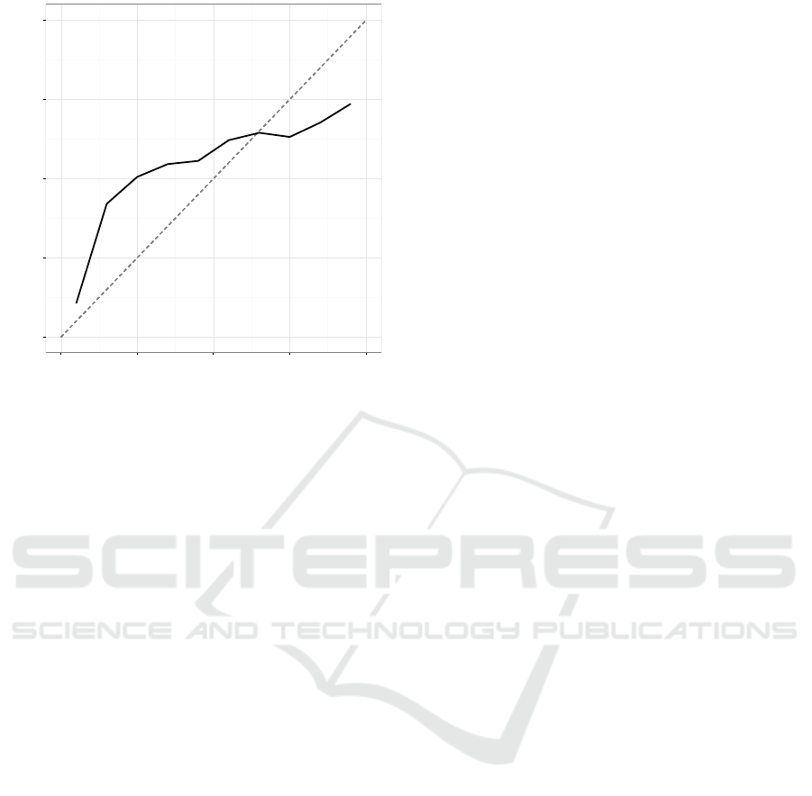
Calibration plot is often used to get a quick glance
at the calibration performance visually. In calibration
plots, test data set predictions are grouped into bins
according to their prediction scores. For each bin, the
fraction of samples belonging to the positive class is
determined. The fraction of positives is then plotted
against the bin center values. If the bin center values
and fraction of positives in the corresponding bins are
close for each bin, the prediction scores are well cal-
ibrated. An example calibration plot can be seen in
ICAART 2018 - 10th International Conference on Agents and Artificial Intelligence
380
●
●
●
●
●
●
●
●
●
●
0.00
0.25
0.50
0.75
1.00
0.00 0.25 0.50 0.75 1.00
Prediction Score
% Positive Class
Figure 1: Calibration plot of the Adult data set classified
with Na
¨
ıve Bayes classifier. The dashed line represents per-
fect calibration.
Figure 1. The amount of data affects calibration plots
as the amount of data in each bin needs to be suffi-
cient to be a representative sample of the general cal-
ibration performance in that prediction score range.
Interpretation of the calibration plot is obviously sub-
jective and does not take into account the distribution
of the prediction scores. It can, however, give valu-
able additional information to the modeler when used
together with error metrics such as MSE and logloss.
4 GENERATING CALIBRATION
DATA
Traditionally, calibration algorithms use a fraction of
the training data set, separate from the data used to
train the classifier, to tune the calibration model to
avoid bias. Often, however, the amount of data avail-
able is limited. In addition, Na
¨
ıve Bayes classifier
tends to push uncalibrated prediction scores towards
the extremes, leaving very little data to be used to tune
the calibration model especially in the middle of the
prediction score range.
If we knew the true probability distribution of our
data, we could construct a perfect Bayesian model for
classification and no calibration would be needed. As
this is not possible in practice, we obviously cannot
use the probability distribution to draw the calibra-
tion data from that, either. To get an estimate of the
data distribution we can fit a classification model to
the training data and use that model to generate more
data that is used for calibration. As was stated above,
the same data cannot, however, be used for training
the model and for calibration to avoid bias. There-
fore, in our approach, the calibration data is gener-
ated with cross-validation within the training data set.
Hence we are not limited to a fraction of the training
data and we can use the whole training data to train
the prediction model which is obviously valuable. Of
course, we cannot generate data out of nowhere but
we argue that with our approach we can make better
use of the existing information in our training data.
4.1 Traditional Approach
For the traditional isotonic regression, 10 % of the
training data was split off to be used as the calibration
data set and the rest was used to train the prediction
model. A completely separate test data set was used
to test the calibration performance.
4.2 Our Approach
In designing our calibration algorithm, two goals
were in mind. First, the effect of training data set size
on the calibration performance was to be reduced, and
second, calibration performance was to be improved
over traditional isotonic regression.
To achieve these goals, cross validation was used
to generate the calibration data set. This generated
data set was made available to the actual calibration
algorithm, isotonic regression in this case. Similar
approach to generate data was used by Alasalmi et al.
(Alasalmi et al., 2016) for classification confidence
estimation. Here we will use the same idea in the case
of calibration. The procedure is shortly described be-
low.
To generate the calibration data set, the training
data was processed in a cross validation manner. 70
% of the training data was used to train a Na
¨
ıve Bayes
classifier and the rest of the training data set was then
predicted with the model. Prediction scores as well
as the true classes of those data points were added
to the calibration data set. This procedure was then
repeated with a different split of the data until at least
the desired number of data, 5 000 samples in this case,
was generated for the calibration data set. About 1
000 samples in the calibration data set has been sug-
gested as the minimum for isotonic regression (Caru-
ana et al., 2008; Niculescu-Mizil and Caruana, 2005).
However, there seems to be improvement in isotonic
regression calibration performance with more data
(Niculescu-Mizil and Caruana, 2005). Therefore we
chose to use 5 000 sample target in our calibration
data generation.
Getting More Out of Small Data Sets - Improving the Calibration Performance of Isotonic Regression by Generating More Data
381

Figure 2 summarizes the proposed algorithm for
generating data for calibration. This generated data
set was then used to train an isotonic regression model
that was used for calibrating the prediction scores of
previously unseen data. We call this the Data Genera-
tion (DG) calibration model. We also wanted to test if
grouping together calibration data points with similar
prediction scores before feeding them into isotonic re-
gression would further increase the calibration perfor-
mance. For this purpose, the 5 000 generated calibra-
tion data points were aggregated into groups of 100
data points and these aggregated data samples were
instead fed to the calibration algorithm. We call this
model the Data Generation and Grouping (DGG) cal-
ibration model. In essence, each aggregated sample
represents an average calibration score and an asso-
ciated fraction of positive samples in the aggregate.
The amount of data points to aggregate into a sample
is a compromise between the resolution of prediction
scores and the resolution of the fraction of positives
in the sample.
Training
data set
Classifier
Train
Predict
Calibration
data set
Figure 2: Calibration data set generation. Cross validation
was repeated until the calibration data set size reached 5 000
samples.
5 EXPERIMENTS
To test the algorithm we developed, an experiment
was set up as follows. Each data set was split into
training and test data sets. 30 % of the samples were
used as the test data while the rest served as the train-
ing data. Using the training data set only, a Na
¨
ıve
Bayes classifier was trained and four different cali-
bration schemes were run using the training data set:
control (no calibration, raw prediction scores), tra-
ditional isotonic regression calibration, and our two
developed algorithms (DG and DGG). For the tradi-
tional isotonic regression, 10 % of the training data
was put aside for calibration and the rest was used to
train the prediction model. For our developed algo-
rithms, cross validation was used to create the sep-
arate calibration dataset, as described in Section 4,
and the whole training data set was used to train
the prediction model. Next, the test data set sam-
ples were predicted and the prediction scores were
calibrated using the algorithms tuned in the previous
step. Threshold value used as prediction boundary
was tuned with the calibrated training data to max-
imize classification rate. This was done separately
for each calibration scheme. Using the threshold
from the previous step as the cut off prediction score,
the following metrics for classification and calibra-
tion performance were calculated for each calibration
scheme: classification rate, logarithmic loss (logloss),
and mean squared error (MSE). For each data set, this
procedure was repeated 10 times with a different split
into training and test data sets and the average perfor-
mance is reported in the results to reduce the amount
of chance in the results.
The experiments were run with the data sets
whose properties are presented in Table 1. All of
the problems were already or were converted into bi-
nary classification problems as described below. The
prediction task with QSAR biodegradation data set
(Mansouri et al., 2013) (Biodegradation) is to clas-
sify chemicals into ready or not ready biodegradable
categories based on molecular descriptors. In Blood
Transfusion Service Center data set (Yeh et al., 2009)
(Blood donation), the task is to predict whether pre-
vious blood donors donated blood again in March
2007. Contraceptive Method Choice data set (Con-
traceptive) is a subset of the 1987 National Indonesia
Contraceptive Prevalence Survey. The prediction task
is to predict the current contraceptive method choice.
A combination of classes short-term and long-term
were used as the positive class while the no-use class
served as the negative class. Letter Recognition data
set (Letter) is a database for letter identification based
on predetermined image features. We used a variation
of the data set by reducing it down into two similar
letters. The letter Q served as the positive class and
the letter O as the negative class. The Mushroom data
set contains descriptions of physical characteristics of
mushrooms and the prediction task is to determine if
the mushrooms are edible or poisonous. All data sets
are freely available from the UCI machine learning
repository (Lichman, 2013).
Comparison of traditional isotonic regression,
Data Generation calibration, and Data Generation and
Grouping calibration algorithms on the Mushroom
data set is shown in Figure 3. Figures 3a-3c show
the traditional isotonic regression, Data Generation,
and Data Generation and Grouping calibration mod-
els, respectively. Also, a calibration plot with the four
calibration algorithms is shown in Figure 3d.
Classification rates (CR), loglosses, and MSEs for
each calibration scheme are presented in Tables 2-6.
ICAART 2018 - 10th International Conference on Agents and Artificial Intelligence
382
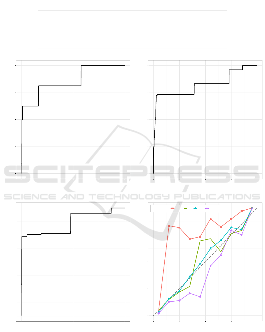
Table 1: Data set properties.
Data set Samples Features Positive class Calibration samples
Biodegradation 1055 41 34 % 73
Blood donation 748 4 24 % 52
Contraceptive 1473 9 57 % 103
Letter 1536 16 51 % 107
Mushroom 8124 20 52 % 568
0.00
0.25
0.50
0.75
1.00
0.00 0.25 0.50 0.75 1.00
Prediction Score
% Positive Class
(a) Traditional isotonic regression model.
0.00
0.25
0.50
0.75
1.00
0.00 0.25 0.50 0.75 1.00
Prediction Score
% Positive Class
(b) Data Generation calibration model.
0.00
0.25
0.50
0.75
1.00
0.00 0.25 0.50 0.75 1.00
Prediction Score
% Positive Class
(c) Data Generation and Grouping calibration model.
●
●
●
●
●
●
●
●
●
●
0.00
0.25
0.50
0.75
1.00
0.00 0.25 0.50 0.75 1.00
Predicted Probability
% Positive Class
Algorithm
●
Raw IR DG DGG
(d) Calibration plot of all calibration schemes.
Figure 3: Calibration models and calibration plot for the Mushroom data set.
Getting More Out of Small Data Sets - Improving the Calibration Performance of Isotonic Regression by Generating More Data
383
The results are reported as average values of 10 sim-
ulations. For logloss and MSE, the lowest values, i.e.
the best calibration result according to that metric, are
in boldface. Statistical significance of the difference
in the mean values was calculated using a Welch t-
test (Welch, 1947) and the significant differences are
indicated in the Tables.
Table 2: Performance metrics on the Biodegradation data
set.
∗
Significantly lower than Raw, p < 0.05.
∗∗
Signifi-
cantly lower than Raw, p < 0.01. † Significantly lower than
IR, p < 0.05. ‡ Significantly lower than IR, p < 0.01.
Algorithm CR Logloss MSE
Raw 84.6 % 13.77 0.570
IR 83.2 % 4.81
∗∗
0.278
∗∗
DG 84.5 % 3.42
∗∗
0.268
∗∗
DGG 84.7 % 0.93
∗∗
‡ 0.246
∗∗
†
Table 3: Performance metrics on the Blood donation data
set.
∗
Significantly lower than Raw, p < 0.05.
∗∗
Signifi-
cantly lower than Raw, p < 0.01. † Significantly lower than
IR, p < 0.05. ‡ Significantly lower than IR, p < 0.01.
Algorithm CR Logloss MSE
Raw 75.8 % 1.49† 0.381
IR 75.4 % 4.17 0.393
DG 75.6 % 1.21
∗∗
‡ 0.342
∗
‡
DGG 75.9 % 1.04
∗∗
‡ 0.343
∗
‡
Table 4: Performance metrics on the Contraceptive data set.
∗
Significantly lower than Raw, p < 0.05.
∗∗
Significantly
lower than Raw, p < 0.01. † Significantly lower than IR,
p < 0.05. ‡ Significantly lower than IR, p < 0.01.
Algorithm CR Logloss MSE
Raw 63.5 % 1.85† 0.515
IR 63.8 % 2.45 0.469
∗∗
DG 63.4 % 1.28
∗∗
‡ 0.450
∗∗
‡
DGG 62.9 % 1.28
∗∗
‡ 0.450
∗∗
‡
6 DISCUSSION
The calibration models for the different calibration
schemes in Figures 3a-3c do not differ dramatically.
The traditional isotonic regression model is more
coarse because of the low amount of data available.
However, as a significant portion of the prediction
scores tend to be near zero and one with Na
¨
ıve Bayes
classifier, the differences in the calibration models
near zero and one can become significant, especially
when logloss is used as the error metric, as we will
see later.
Table 5: Performance metrics on the Letter data set.
∗
Sig-
nificantly lower than Raw, p < 0.05.
∗∗
Significantly lower
than Raw, p < 0.01. † Significantly lower than IR, p < 0.05.
‡ Significantly lower than IR, p < 0.01.
Algorithm CR Logloss MSE
Raw 83.3 % 1.16 0.295
IR 82.3 % 1.68 0.239
∗∗
DG 83.2 % 0.72
∗∗
‡ 0.222
∗∗
DGG 83.0 % 0.72
∗∗
‡ 0.223
∗∗
Table 6: Performance metrics on the Mushroom data set.
∗
Significantly lower than Raw, p < 0.05.
∗∗
Significantly
lower than Raw, p < 0.01. † Significantly lower than IR,
p < 0.05. ‡ Significantly lower than IR, p < 0.01.
Algorithm CR Logloss MSE
Raw 97.4 % 0.359 0.081
IR 97.2 % 0.376 0.046
∗∗
DG 97.4 % 0.192
∗∗
‡ 0.043
∗∗
DGG 97.1 % 0.223
∗∗
‡ 0.044
∗∗
Visually inspected (Figure 3d), calibration of raw
Na
¨
ıve Bayes prediction scores with the Mushroom
data set is not very good. However, all of the com-
pared calibration algorithms were able improve the
calibration with this data set based on the calibration
plot. Based on the plot, DG calibration seems to per-
form best, i.e. it runs overall closest to the center line
meaning that the predicted probability and the true
fraction of positives are well correlated.
More objective measures for calibration perfor-
mance are logloss and MSE. With only one of the data
sets, traditional isotonic regression was able to im-
prove the calibration of Na
¨
ıve Bayes when using the
logarithmic loss as the measure of calibration perfor-
mance. On the other four data sets, however, logloss
actually increased compared to the uncalibrated con-
trol although in two cases the difference was not sta-
tistically significant. This is not very surprising be-
cause the calibration data sets were very small and
isotonic regression needs a decent amount of data
to work properly in calibration without overfitting.
On the other hand, by generating more data to be
used for calibration, as suggested in this article, the
logloss was lower with every tested data set than with
raw prediction scores or prediction scores calibrated
with traditional isotonic regression, sometimes dras-
tically. The differences were statistically significant
in every case when compared to uncalibrated con-
trol. When compared to isotonic regression, the dif-
ferences were statistically significant with the excep-
tion of DG model on the Biodegradation data set.
When using the mean squared error metric for cal-
ibration success, it seems that isotonic regression may
ICAART 2018 - 10th International Conference on Agents and Artificial Intelligence
384
be able to improve the calibration over raw predic-
tion scores in most cases. More specifically, MSE
for isotonic regression was statistically significantly
lower than than uncalibrated control with the excep-
tion of the Blood donation data set. By generating
more calibration data we were able to decrease MSE
with every tested data set and the differences were
statistically significant in all cases for both DG and
DGG model when compared to uncalibrated control.
MSE with both DG and DGG were statistically signif-
icantly lower than with isotonic regression on Blood
donation and Contraceptive data sets as well as for
DGG on the Biodegradation data set.
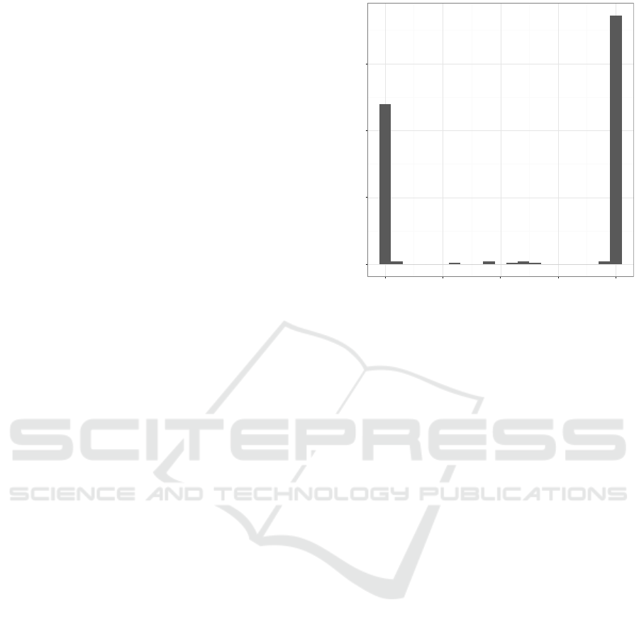
Data sets with prediction scores that are very
much pushed towards one and zero suffer from an un-
expected problem regarding calibration. As the algo-
rithm that is used to produce the isotonic regression
function cannot handle several data points with the
same prediction score, much of the calibration data
can be lost and wrong conclusions can be made, es-
pecially on the smaller data sets. This can lead to
mistakes in calibration particularly near one and zero
where logloss will penalize errors hard. MSE, how-
ever, is not as much affected by the errors made in
the extreme ends. The Biodegradation data set is one
example of such problem. Histogram of the raw pre-
diction scores with this data set is depicted in Fig-
ure 4. Our Data Generation and Grouping model tries
to address this issue by aggregating calibration data
into larger samples and averaging them. DGG per-
forms best of all of the algorithms with the problem-
atic Biodegradation data set and on par with DG on
three other data sets. On the Mushroom data set DG
works better than DGG, although the difference in
logloss is not statistically significant. However, DGG
can still beat uncalibrated prediction scores and tradi-
tional isotonic regression calibration by a clear mar-
gin. This result is somewhat surprising as we were
using groups of 100 data points resulting in only 50
samples in the calibration data set which is actually
smaller calibration data set than in any of the tested
data sets. These samples better represent the true na-
ture of the data set than the same amount of individual
data points can.
It is impossible, of course, to correct for shortcom-
ings of the data set itself just by sampling but we argue
that our approach makes it possible to make better use
of the data that is available. This is apparent from the
error metrics. Clearly, using a very small data set for
calibration can not be advised based on our results, as
has been suggested in the literature, too. But gener-
ating more calibration data with either DG or DGG
model can lower error metric figures indicating the
calibration function is less biased towards the calibra-
0
50
100
150
0.00 0.25 0.50 0.75 1.00
Prediction Score
Count
Figure 4: Histogram of the raw prediction scores in an ex-
treme example, the Biodegradation data set.
tion data set making it better generalized for unseen
data.
The different calibration schemes do not have any
significant effect on classification rate. This is ex-
pected as ranking of the predictions is not affected by
calibration if the original ranking was somewhat close
to being correct.
Classification rate is inversely associated with
both logloss and MSE. This is because a correct clas-
sification will always lead to a smaller error than
an incorrect one, however uncertain it was to begin
with. The small differences in classification rate be-
tween calibration conditions cannot, however, explain
the lower error metrics achieved with the calibration
schemes. The differences are, therefore, explained by
the performance differences between the tested cali-
bration algorithms.
7 CONCLUSIONS
Small data sets are problematic for isotonic regression
calibration and applying it might actually worsen the
calibration of unseen data. Making better use of the
information in the data by generating more calibra-
tion data can alleviate the problem. With the approach
suggested in this article, we were able to improve cal-
ibration of Na
¨
ıve Bayes over uncalibrated and tradi-
tional isotonic regression with every tested data set.
In some cases, grouping the generated calibration data
into small samples can lead to even better calibration
than just using the generated data intact. Generat-
ing the calibration data is obviously computationally
Getting More Out of Small Data Sets - Improving the Calibration Performance of Isotonic Regression by Generating More Data
385

more complex than just splitting the training data set
in two. The actual computational cost will depend on
the classification model used. However, the calibra-
tion data generation only needs to be done once in the
training phase and obtaining the calibrated prediction
score for new data is very fast.
If the amount of training data available is limited
and a good calibration of the used classifier is impor-
tant, using the suggested approach for calibration can
be a viable option.
ACKNOWLEDGEMENTS
The authors would like to thank Infotech Oulu, Jenny
and Antti Wihuri Foundation, and Tauno T
¨
onning
Foundation for financial support of this work.
REFERENCES
Alasalmi, T., Koskim
¨
aki, H., Suutala, J., and R
¨
oning, J.
(2016). Instance level classification confidence esti-
mation. In Advances in Intelligent Systems and Com-
puting. The 13th International Conference on Dis-
tributed Computing and Artificial Intelligence 2016,
pages 275–282. Springer.
Caruana, R., Karampatziakis, N., and Yessenalina, A.
(2008). An empirical evaluation of supervised learn-
ing in high dimensions. In Proceedings of the 25th In-
ternational Conference on Machine Learning, ICML
’08, pages 96–103. ACM.
Domingos, P. and Pazzani, M. (1997). On the Optimality of
the Simple Bayesian Classifier under Zero-One Loss.
Machine Learning, 29:103–130.
Kononenko, I. (1990). Comparison of inductive and naive
bayesian learning approaches to automatic knowledge
acquisition. Current trends in knowledge acquisition,
pages 190–197.
Kuhn, M. and Johnson, K. (2013). Applied Predictive Mod-
eling. New York: Springer.
Lichman, M. (2013). UCI Machine Learning Repository
http://archive.ics.uci.edu/ml. University of California,
Irvine, School of Information and Computer Sciences.
Mansouri, K., Ringsted, T., Ballabio, D., Todeschini, R.,
and Consonni, V. (2013). Quantitative structure–
activity relationship models for ready biodegradability
of chemicals. Journal of Chemical Information and
Modeling, 53(4):867–878.
Niculescu-Mizil, A. and Caruana, R. (2005). Predicting
good probabilities with supervised learning. In Pro-
ceedings of the 22Nd International Conference on
Machine Learning, ICML ’05, pages 625–632. ACM.
Welch, B. L. (1947). The generalization of student’s prob-
lem when several different population variances are
involved. Biometrika, 34(1-2):28–35.
Yeh, I.-C., Yang, K.-J., and Ting, T.-M. (2009). Knowledge
discovery on {RFM} model using bernoulli sequence.
Expert Systems with Applications, 36(3, Part 2):5866
– 5871.
Zadrozny, B. and Elkan, C. (2002). Transforming classifier
scores into accurate multiclass probability estimates.
In Proceedings of the Eighth ACM SIGKDD Interna-
tional Conference on Knowledge Discovery and Data
Mining, KDD ’02, pages 694–699. ACM.
Zhang, H. and Su, J. (2008). Naive bayes for optimal rank-
ing. Journal of Experimental & Theoretical Artificial
Intelligence, 20(2):79–93.
Zhong, L. W. and Kwok, J. T. (2013). Accurate probability
calibration for multiple classifiers. In Proceedings of
the 13th International Joint Conference on Artificial
Intelligence, IJCAI ’13, pages 1939–1945.
ICAART 2018 - 10th International Conference on Agents and Artificial Intelligence
386
