The Shape of an Image

A Study of Mapper on Images

Alejandro Robles

, Mustafa Hajij

and Paul Rosen

Department of Electrical Engineering, University of South Florida, Tampa, U.S.A.

Department of Computer Science and Engineering, University of South Florida, Tampa, U.S.A.

Keywords:

Mapper, Contour Tree, Topological Data Analysis.

Abstract:

We study the topological construction called Mapper in the context of simply connected domains, in particular

on images. The Mapper construction can be considered as a generalization for contour, split, and joint trees on

simply connected domains. A contour tree on an image domain assumes the height function to be a piecewise

linear Morse function. This is a rather restrictive class of functions and does not allow us to explore the topology

for most real world images. The Mapper construction avoids this limitation by assuming only continuity on the

height function allowing this construction to robustly deal with a signiﬁcantly larger set of images. We provide

a customized construction for Mapper on images, give a fast algorithm to compute it, and show how to simplify

the Mapper structure in this case. Finally, we provide a simple procedure that guarantees the equivalence of

Mapper to contour, join, and split trees on a simply connected domain.

1 INTRODUCTION

Recently, the study of data has beneﬁted from the

introduction of topological concepts (Carlsson, 2009;

Carlsson et al., 2008; Carlsson et al., 2005; Collins

et al., 2004), in a process known as Topological Data

Analysis (TDA).

One of the most successful topological tools for

shape analysis is the contour tree (Boyell and Ruston,

1963). The contour tree of a scalar function, deﬁ-

ned on a simply connected domain, can be thought of

as an efﬁcient topological summary of that domain.

This structure is obtained by encoding the evolution of

the connectivity of the level sets induced by a scalar

function deﬁned on the domain. Contour trees are of

fundamental importance in computational topology,

geometric processing, image processing and computer

graphics.

Contour trees are particularly useful for processing

massive data. Contour trees, and their more general

version Reeb graphs (Reeb, 1946), have been used

in numerous applications including shape understan-

ding (Attene et al., 2003), visualization of isosurfa-

ces (Bajaj et al., 1997), contour indexing (Boyell and

Ruston, 1963), image processing (Kweon and Kanade,

1994), data simpliﬁcation (Carr et al., 2004; Rosen

et al., 2017b), and many other applications. Contour

tree algorithms can be found in many papers such as

(Takahashi et al., 2009; Rosen et al., 2017a) and Reeb

graphs algorithms are studied in (Shinagawa and Kunii,

1991; Doraiswamy and Natarajan, 2009).

Singh et al. proposed a method to understand the

shape of data using a topology-inspired construction

called Mapper (Singh et al., 2007). Since then, Mapper

has became one of the most popular tools used in TDA.

It has been applied successfully for various data related

problems (Lum et al., 2013; Nicolau et al., 2011) and

studied from multiple points of view (Carri

ere and

Oudot, 2015; Dey et al., 2017).

The construction of Mapper is closely related to

Reeb graphs and contour trees (Singh et al., 2007).

Indeed this construction can be considered as a genera-

lization of Reeb graph under some technical conditions

(Munch and Wang, 2015). The relation between Reeb

graph and Mapper has recently been made precise in

(Carri

ere and Oudot, 2015).

The true power of Mapper lies in its general des-

cription in terms of topological spaces and maps on

them. This abstract version of the construction is usu-

ally called topological Mapper. In the original work

where Mapper was introduced (Singh et al., 2007),

Mapper was applied to study the shape of point clouds.

This version of Mapper is now referred to as statistical

Mapper (Stovner, 2012). While topological Mapper

allows one to introduce the main ideas of Mapper in

general terms, statistical Mapper deals with aspects

Robles, A., Hajij, M. and Rosen, P.

The Shape of an Image - A Study of Mapper on Images.

DOI: 10.5220/0006574803390347

In Proceedings of the 13th International Joint Conference on Computer Vision, Imaging and Computer Graphics Theory and Applications (VISIGRAPP 2018) - Volume 4: VISAPP, pages

339-347

ISBN: 978-989-758-290-5

339

related to point clouds, such as clustering and noise.

Similar technical aspects arise when trying to apply

Mappers on other domains, such as images.

The purpose of this article is to study Mapper on

speciﬁc domains, namely simply connected domains

and apply this study to images. While the focus of this

article is Mapper on images, we state the results whe-

never possible on a general simply connected domain.

1.1 Contribution

Mapper construction on images operates on a height

function deﬁned on the image domain. The height

function can be a color channel or luminance of the

input image itself or the gradient magnitude of the

image, which is typically a compact and connected

region in

. After discussing the topological and

statistical versions of Mapper construction on image

domains, we relate this construction to the contour

tree algorithm that enables Mapper to realize contour,

merge, and split trees.

The method we propose here has multiple advan-

tages. Beside being theoretically justiﬁed, the con-

struction of Mapper is ﬂexible and applicable to conti-

nuous scalar function deﬁned on a simply connected

domain in any dimension. Contour tree algorithms on

simply connected domains assume the height function

on the domain to be piecewise linear Morse function.

While this class of function is useful for a wide vari-

ety of applications, it is rather restrictive for images

and it does not allow us to explore the topology for

most real world images without heavy preprocessing

of the image height function. Mapper construction

avoids this limitation by assuming only continuity on

the height function allowing this construction to ro-

bustly deal with a signiﬁcantly larger class of images.

Moreover, Mapper naturally gives a multi-resolution

hierarchical understanding of topology of the under-

lying domain.

The approach we take to Mapper here is geared for

simply connected domains and, in particular, for ima-

ges. Using the properties of such domains, we provide

a fast construction algorithm. Finally, we provide a

simple algorithm that guarantees the equivalence of

Mapper construction to contour, join, and split trees

on a simply connected domain.

2 PRELIMINARIES AND

MOTIVATION

As mentioned in the introduction, Mapper is closely

related to the contour tree. This related structure moti-

vates the construction of Mapper.

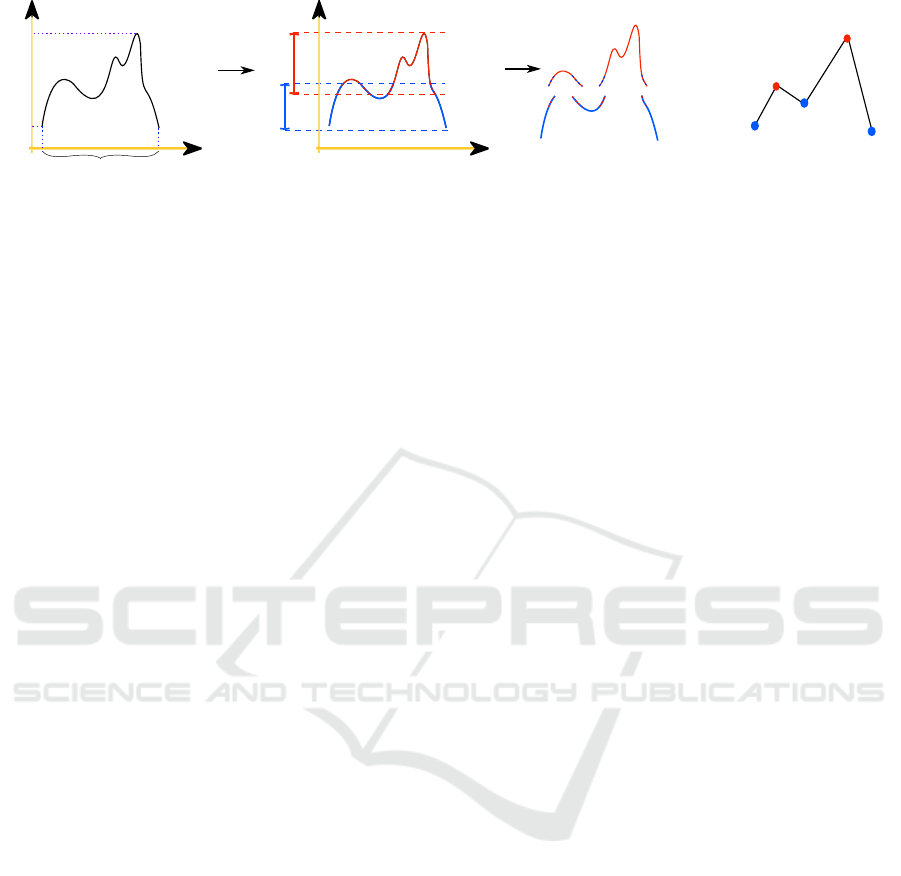
(c)(b)(a) (d)

Figure 1: (a) Scalar function is segmented into (b) topologi-

cal regions by converting that scalar ﬁeld into a (c) landscape,

using the intensity value for height. The connection of those

regions can be converted into a contour tree (d) that describes

the topology.

Contour Trees.

The contour tree of a scalar ﬁeld, de-

ﬁned on a simply connected domain, tracks the evolu-

tion of contours in that ﬁeld and stores this information

in a tree structure. Each node in the tree represents a

critical point where contours appear, disappear, merge,

or split. Each edge corresponds to adjacent and topo-

logically equivalent contours. In essence, the contour

tree forms a topological skeleton that connects critical

points (i.e. local minima, maxima, and saddle points).

Figure 1 shows an example of the contour tree of a

scalar ﬁeld deﬁned on a 2d domain.

In practice, we usually want to compute contour

trees on a piecewise linear Morse function deﬁned on

a simplicial complex. The mathematical framework

speciﬁed for contour tree does not apply directly on

such domains. The difﬁculty rises when one tries

to extract isosurfaces for a scalar value as the pre-

images of an scalar values may not be an isosurface

(Szymczak, 2005). Nonetheless several contour tree

algorithms have been proposed, but they all depend

some method of isosurface extraction. Hence two

different methods of isosurface extraction might lead

to two different contour trees.

Mapper.

The construction of Mapper avoids the pro-

blem of dealing with isosurfaces all together by fo-

cusing on portions of the range of the scalar ﬁeld.

To illustrate this, consider the simple scalar function

f : X −→ [a, b]

example given in Figure 2. Cover

the range

[a, b]

by two overlapping intervals

A :=

(a −ε, c + ε)

and

B =: (c − ε, b + ε)

such that

c ∈ [a, b]

and

ε > 0

. Note the interval

and

cover the interval

[a, b] in the sense : [a, b] ⊂ A ∪ B.

Now, consider the inverse images

−1

(A)

and

−1

(B)

. Figure 2 (c) illustrates that

−1

(A)

consists of

two connected components

and

−1

(B)

con-

sists of a three connected components

and

Moreover, there are some overlaps between these con-

nected components. Namely, the intersections

∩ β

∩β

and

∩β

are non-empty. We record

the information of the connected components and their

VISAPP 2018 - International Conference on Computer Vision Theory and Applications

340

A α

(a) (b) (c) (d)

Figure 2: The construction of Mapper on a 1d function. (a) A scalar function

f : X −→ [a, b]

. (b) The range

[a, b]

is covered by

the two intervals A, B. (c) This gives a decomposition of the domain X. (d) Mapper is constructed.

non-empty overlap by a graph structure. The nodes of

this graph represent the connected components and the

edges represent the non-empty intersection between

these components. The Mapper construction is the

graph associated to the function

and the cover

A, B

in this manner.

Mapper’s Relationship to Contour Trees.

One

can notice that this graph is very related to the contour

tree. Both the contour tree and Mapper essentially

track the same topological information in the scalar

ﬁeld, but the way this information is encoded in each

one of them is different. The nodes of the contour

tree of a scalar ﬁeld are represented by the critical

points the ﬁeld and the edges represent the regions in

the domain where the are no topological change in

the contours. On the other hand the nodes in Map-

per represent connected regions in the domain and the

edges represent the connection between two different

connected components. Hence, the combination stores

when a topological change occur to the contour.

3 TOPOLOGICAL MAPPER

We now give the general deﬁnition of Mapper for a

continuous scalar function deﬁned on a simply con-

nected domain.

Let

be a simply connected domain in

. We

will assume that

is compact and connected. A cover

is a collection of open sets

U = {U

}

i∈I

such

that

X ⊂ ∪

i∈I

here is any indexing set. The com-

pactness condition implies that we can always ﬁnd

a ﬁnite cover for

. In the case of an image,

is a

compact simply connected subset of

. The

nerve

(U, X )

induced by the covering of

is a

graph with nodes are represented by the elements of

and edges represented by the pairs

A, B

such that

A ∩ B 6=

. The nerve of a space

can be thought of

as a topological skeleton of the underlying space. The

main idea of Mapper lies in the way of constructing

this cover using the range of a function

deﬁned

. More precisely, a continuous scalar function

f : X −→ [a, b]

and a cover for the range of

give rise to a natural cover of

in the following way. A

cover for an interval

[a, b]

is ﬁnite collection of open in-

tervals

U = {(a

, b

), ..., (a

, b

)}

that cover

[a, b]

, i.e.

[a, b] ⊂ ∪

i=1

, b

)

. Now take the inverse images of

each open set in

under the function

. The result is

U( f ) := { f

−1

((a

, b

)), ..., f

−1

((a

, b

))}

is an open

cover for the space

. The open cover

U( f )

can now

be used to obtain the

-nerve graph

M(X, f , U) :=

(X, U( f ))

. The Mapper construction is by deﬁni-

tion the graph M(X, f , U).

3.1 Cover Resolution

For a ﬁxed function

the graph

M(X, f , U)

depends

on the choice of the cover

of the interval

[a, b]

. This

idea of Mapper resolution can be made precise via

the notion of cover reﬁnement (Munkres, 2000). Let

be a space and let

and

be two covers of

The cover

is a reﬁnement a cover

if for each

element of

there is at least one element

such that

B ⊆ A

. If

is a reﬁnement a cover

there is a embedding of the graph

(X, A)

inside the

graph

(X, B)

. That is there is one-to-one function

that maps between the vertices sets

(X, A)

and

(X, B)

together with an assignment that assigns to

every edge

e = (u, v)

(X, A)

a path in

(X, B)

between

φ(u)

and

φ(v)

. See (Munkres, 2000). Figure 8

show examples

nested sequences of cover reﬁnement

along with their corresponding graphs. This simple,

effective, way to give a multi-resolution Mapper is one

of its main advantages over contour tree.

4 TOPOLOGICAL MAPPER ON

IMAGES

In this section, we discuss the details of topologi-

cal Mapper on images that will be used in our algo-

The Shape of an Image - A Study of Mapper on Images

341

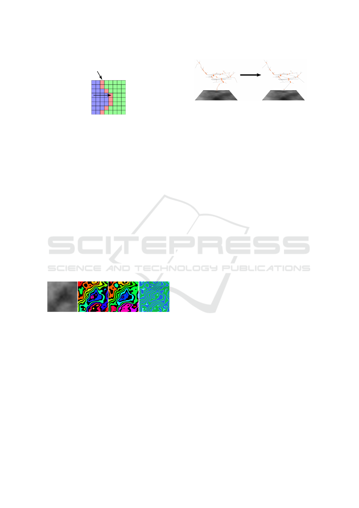
Figure 3: The two types of pixel adjacency relation.

rithm for the statistical Mapper on images discussed

in section 5. We assume that

f : X −→ [a, b]

is con-

tinuous height function deﬁned on the image domain

X ⊂ R

4.1 Choosing the Cover

While the choice of cover for the Mapper construction

is ﬂexible, certain covers that give rise to a non-

desirable tree structure. We describe an effective way

to construct the cover for the domain that will help in

computing Mapper efﬁciently.

Start by splitting the interval

[a, b]

into n subin-

tervals

, c

], [c

, c

], ..., [c

n−1

, c

]

such that

= a

and

= b

. Choose

ε > 0

and construct a cover

U(ε, n) = {U

= (c

− ε, c

i+1

− ε)}

n−1

i=1

for the inter-

val

[a, b]

. We want to choose

so that only adjacent

intervals intersect. The choice of

should satisﬁes the

following conditions:

The intersection

∩U

unless

j ∈ {i − 1, i, i +

1} for 2 ≤ i, j ≤ n − 2.

2. U

∩U

unless

j ∈ {1, 2}

and ﬁnally

n−1

∩

0 unless j ∈ {n − 2, n − 1}.

This choice of

ensures that only adjacent inter-

vals intersect with each other. We denote

odd

to the

subset of

consisting of intervals with odd indices.

Similarly we deﬁne

even

to be the collection of open

sets

∈ U

such that index

is even. These cover

choices minimize the number of overlaps between the

cover elements.

4.2 Determining the Nodes

A node in Mapper is a connected component of

−1

((c, d))

, where

(c, d)

is an open interval in the

cover

of the range of

. Given a range

(c, d)

, in the

case of an image

, we want to ﬁnd the those pixels in

whose pixel value lie in

(c, d)

. Given a region

an image

consisting of a collection of pixels whose

pixel value lie within the range

(a, b)

, we want to de-

termine the connected components in the

. Here one

needs to specify what exactly is meant by a connected

component in this context. The image

induces a

graph structure with nodes being the pixels and the

edges are determined by the local pixel adjacency rela-

tion. There are two common types of pixel adjacency

relations shown in Figure 3.

Using the graph on an image with either one

of the pixel adjacency relation conventions, we can

now consider the connected components of subgraph

consists of the pixels in a region

. A walk on

a graph

is a sequence of vertices and edges

, e

, v

, e

, ··· , e

l−1

, v

)

such that

= [v

i−1

, v

] ∈

E(G)

. A graph is said to be connected if there is a

walk between any two vertices. A connected compo-

nent in a graph is a maximal connected subgraph. Fin-

ding connected components of a graph is well-studied

in graph theory and it can be found by in linear time

using either breadth-ﬁrst search or depth-ﬁrst search

(Hopcroft and Tarjan, 1971).

4.3 Determining the Edges

An edge in Mapper is created whenever two connected

components have non-trivial intersection. The cover

that we described for the range

[a, b]

in section 4.1 was

chosen to minimize the number of sets we check for

intersection. Namely the condition that we impose

on the cover of

[a, b]

ensures that only adjacent open

interval overlap. In other words, if

and

are two

open sets in the cover of

U(ε, n)

of the interval

[a, b]

then by the choice of the cover speciﬁed in section 4.1,

we check if the connected components of

−1

)

and

−1

)

intersect only when we know that

and

are adjacent to each other. This signiﬁcantly reduces

the number of set intersections checked.

5 ALGORITHM

The creation of the Mapper graph is done in three

stages. First, all pixels in the image are labeled by the

cover they map to. Pixels with the same label are then

grouped by searching for all connected components

with the same label. This provides the nodes for the

Mapper graph. Next, the connected component regions

are scanned for overlaps. Every pair of overlapping

regions in the image corresponds to an edge connecting

the nodes in the Mapper graph. Finally, the third stage

simpliﬁes the Mapper graph by removing nodes with

two valencies.

5.1 Node Finding

In our approach, pixel labeling is done using a pair of

lookup tables, one for the even cover

even

and one for

the odd cover

odd

. When a lookup table maps outside

of its set of covers, it returns a value that signiﬁes that

VISAPP 2018 - International Conference on Computer Vision Theory and Applications

342

Region 1

Region 2

Candidate Pixels

in Region 2

Figure 4: Line scanning for candidate pixels.

the pixel does not map to a cover in this table. This

even/odd separation has an important beneﬁt that when

one lookup table is applied to the image, none of the

resulting regions overlap. This means that instead of

processing the image for each covering one-by-one,

the image only needs to be processed twice, once for

even

and once for

odd

, to ﬁnd all the connected

regions.

Breadth-ﬁrst search (BFS) is used to ﬁnd connected

regions once the pixels have been labeled. By taking

advantage of the queue structure of BFS, every pixel

in a connected region can be traversed before moving

onto the next region as long as only the top of the

queue is being modiﬁed. This continuity of the search

allows us to add pixels in other regions to the same

queue, thus allowing processing many regions with

one search. As a region is traversed, pixels are marked

with an identiﬁcation unique to that region. In our

implementation, this identiﬁcation is created using the

position of the ﬁrst pixel in the region touched during

the search.

Input EvenOdd Overlap

Figure 5: Region search is done twice, once for even and

once for odd covers. Here, each region identiﬁed during the

search is given a unique color. If a pixel is not found to map

to a cover during the search the, pixel is not colored (these

are the pixels colored in black in the middle two images).

This shows how splitting the covers gives a pair of images

which do not contain overlapping regions. Regions in one

image will, however, overlap with regions in the other image,

as shown in the image on the bottom right.

Our approach initializes the BFS queue with can-

didate pixels which are pixels found by scanning each

row in the image from left to right until a pixel, which

differs in label from the previous pixel is found (see

Figure 4). This gives the pixels that start a region along

every line in the image. Since a region needs at least

one pixel to be in the queue at the start of the search,

the use of candidate pixels ensures each region in the

Figure 6: Simpliﬁcation of the mapper graph.

image will be traversed, while reducing the number of

pixels in the queue at the start of the search.

At the end of the search, every pixel will have an

associated identiﬁcation that represents the connected

component region it belongs to. Finally, these regions

deﬁne the nodes in the Mapper graph. See Figure 5

for illustration of the process of node ﬁnding done on

an example image.

5.2 Edge Finding

Once the regions in the image have been identiﬁed

for both the even and odd covers, overlaps between

regions need to be found. A naive approach would be

to create a set of pixel locations for every region in

both sets of coverings, and check whether pairs of sets

are disjoint. This type of approach, however, requires

every pair of sets to be tested for disjointness, making

it inefﬁcient.

To determine region overlap, we take advantage

of the candidate pixels found during node ﬁnding, see

Figure 4. Since these pixels signiﬁes the entrance of a

region with a different labeling, this means that there

are two different regions from the two opposing covers

overlap. Notice that this method takes advantage of

the way we construct the cover in section 4.1.

5.3 Graph Simpliﬁcation

The resulting Mapper graph can contain thousands

of nodes. Many of these nodes can be removed as

they do not indicate topological events. In the Mapper

graph, a node with valency equal to

corresponds to

a region where no topological event occur. In other

words, such a node is not a merge, split, creation, or

termination of a region. These nodes are analogous to

regular points in the contour tree. Hence, these nodes

can be safely removed to obtain a simpliﬁed graph,

such as in Figure 6.

6 REALIZING THE CONTOUR

TREE

The Mapper construction can be used to realize the

contour tree. Here we give a choice of covering that

The Shape of an Image - A Study of Mapper on Images

343

guarantees that Mapper gives rise to all the topological

information encoded in the contour tree. We need to

assume that the given function is a piecewise linear

Morse function

f : X −→ [a, b]

on a simply connected

domain

. The assumption of piecewise linear Morse

is necessary in order to work with a contour tree. For

precise deﬁnitions related to Morse theory on simpli-

cial complex see (Pascucci et al., 2004).

Recall that every node in the contour tree corre-

sponds to a critical point. The critical point of a

function signiﬁes a topological change in the space

with respect the scalar function. Moreover, if

and

are two consecutive critical values

then for

any two values

, c

∈ (t

)

the number of connected

components of both

−1

)

and

−1

)

are the same.

In other words, a topological change that occur to the

space only when as we sweep though a critical value.

Hence, in order for Mapper to give us the information

encoded in the contour tree, it is sufﬁcient to make a

choice of the covering on

[a, b]

, so that we store the

following information:

The number of connected components between

every two consecutive critical values of f .

The way the connected components merge, split,

appear, and disappear when passing through a cri-

tical point.

The following procedure gives a choice of covering

for [a, b] that satisﬁes the previous two criteria:

Let

, ...,t

be the critical values for

ordered

in an ascending order. Let

, p

, ..., p

be the

corresponding critical points of f .

For each

1 ≤ i ≤ n − 1

, we choose four numbers

, c

and

in the interval

i+1

]

such that

< c

< b

3. Let c

= a − ε and let d

= b + ε for some ε > 0.

Let

be the covering of

[a, b]

consisting of

the intervals

, b

), ..., (a

n−1

, b

n−1

)

as well as

, d

),(c

, d

),...,(c

n−1

, d

Notice that the Mapper construction obtained using

the covering

stores all the topological information

encoded in the function

. Hence, any further reﬁne-

ment of the covering

will not produce any further

details in the Mapper construction as far as the topo-

logy of the original domain is concerned. In other

words, the above construction gives the highest Map-

per resolution that one could obtain on a piecewise

linear Morse function.

7 JOIN AND SPLIT TREES

The previous sections describe how Mapper can be

used to obtain a contour tree. The Mapper construction

is general and can be used to realize other structures

such as the join and split trees (Carr et al., 2003).

The only change one needs to make to the previous

setup is making a different choice for the shape of the

open interval that makes covering of the range. These

choices will be justiﬁed after we illustrate the basic

ideas of join/split trees.

For a continuous scalar function

f : X −→ [a, b]

deﬁned on a simply connected domain

the split tree

ST ( f , X)

tracks the topological changes

occur of the set

{p ∈ X | f (p) ≥ c}

of a value

as this

value is swept from

∞

−∞

. Similarly, the join tree

JT ( f , X)

tracks the topological changes

occur to the topology of the set

{p ∈ X| f (p) ≤ c}

the value

goes from

−∞

∞

. The Mapper con-

struction can be used to compute both split and join

trees on any simply connected domain. The only thing

that must be chosen to obtain these structures is the

shape of the open intervals for the covering

of range

[a, b].

The choice of covering for a join tree should be

of a collection of open intervals of the form

(−∞, c)

that covers the interval

[a, b]

. That is, the cover

must be a ﬁnite set

{(−∞, c

), ..., (−∞, c

)}

such that

[a, b] ⊂ ∪

i=1

(−∞, c

)

. As the values to

increases,

only merging events occur in the set

{p ∈ X| f (p) ≥ c}

which is reﬂected in the resulting Mapper graph. On

the other hand, the choice of covering needed to con-

struct the split tree is a collection of open intervals of

the form (c, ∞).

8 RESULTS

To demonstrate how our work performs we run a few

experiments on some images with various complexi-

ties. Figure 7 shows the illustrative examples on some

images. The height functions chosen on these images

are the input images themselves. The ﬁgure shows

the images along with the Mapper graph on drawn on

the top of them. The vertical position of the node is

chosen to be the average of the pixel values of the re-

gion that corresponds to that node. On the other hand

the

(x, y)

position of a node is the center mass of the

pixel positions of the pixels in the region. The size of

the node is proportional to the number of pixels in the

corresponding connected component.

In Figure 8 we show how multiple reﬁnement of

covering give rise to a hierarchy of Mapper on the

same image. The graphs in the ﬁgure, shown from left

VISAPP 2018 - International Conference on Computer Vision Theory and Applications

344

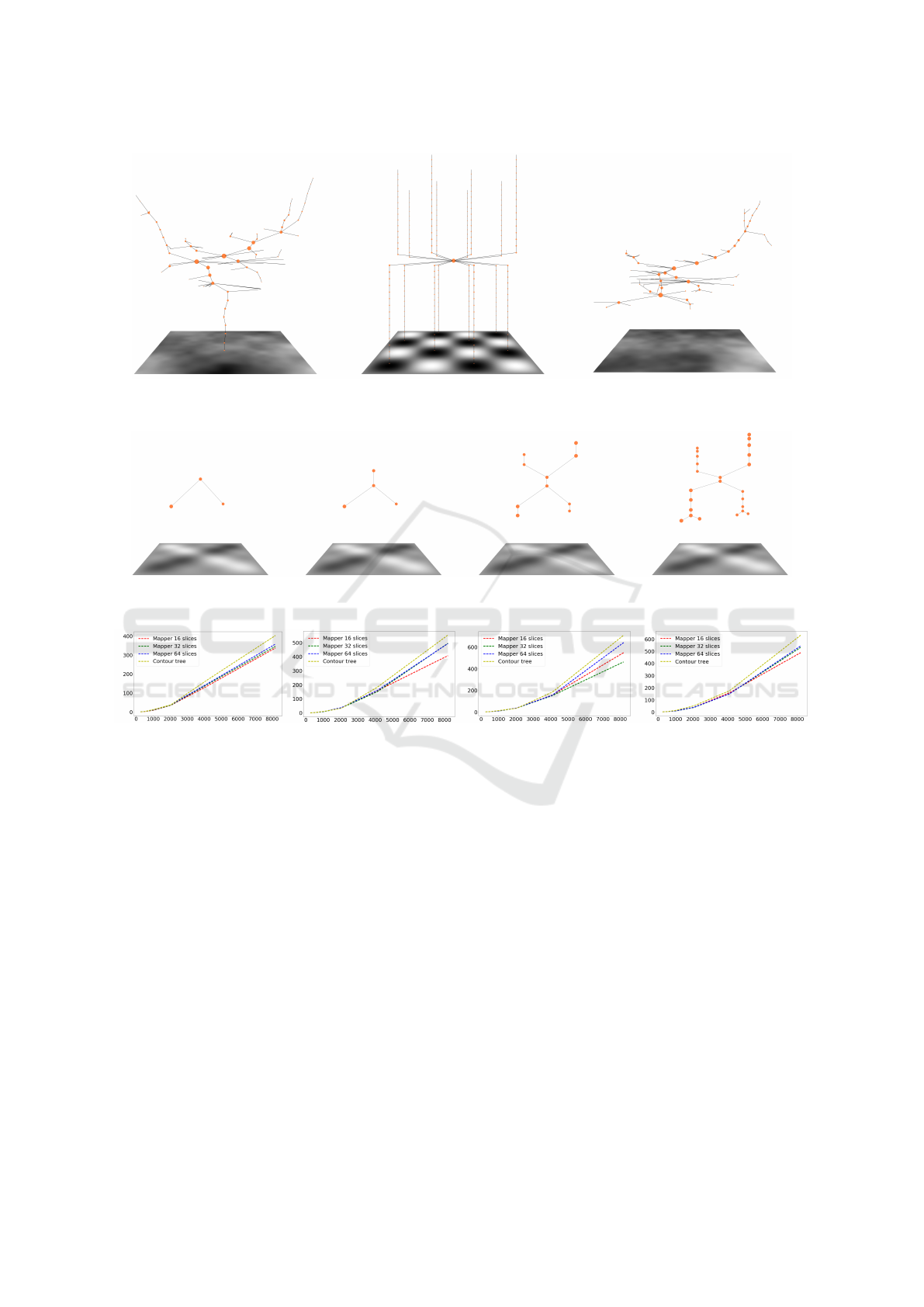
Figure 7: Examples of Mapper on images using pixel values as the height function. The range of these images was covered by

a cover of 32 open sets.

Figure 8: Multi-resolution of Mapper using different covering resolutions. The graphs are constructed from left to right by

using 2, 4, 8, 16 slices of the range covering.

Figure 9: Performance analysis of Mapper in comparison with contour tree on procedurally and non-procedural images. Each

image was done with the resolutions :

256

, 512

, 1024

, 2084

, 4096

and

8192

. Each resolution was tested against Mapper

and contour tree. Mapper was tested using

, and

cover slices. The

-axis represents the square root of the resolution of

the image. The y-axis represents the running time in milliseconds.

to right, are generated by using

2, 4, 8, 16

slices of the

covering. The ﬁgure shows immediately the effect of

cover reﬁnement of the resolution and level of details.

8.1 Running Time

We tested our algorithm on a

3.7

GHs AMD with

GB of memory. We implemented the results

shown in Figures in Java and tested them on the Win-

dows platform. We tested the running time of the

algorithm against two parameters : changing number

of slices in the covers and increasing the resolution of

the image. We performed the tests on procedural and

non-procedural images. See Figure 9 for the perfor-

mance analysis. We also ran a comparison between

the Mapper algorithm we present here and a contour

tree algorithm. The contour tree algorithm we used is

a version of algorithm given in (Carr et al., 2003).

While both contour tree and Mapper give almost

identical performance for images with small resoluti-

ons, Mapper outperforms contour tree as we increase

the resolution of on the image. See Figure 9.

One can notice here that the performance computa-

tion time of Mapper increase linearly with the increase

of number of slices in the cover. Moreover, observe

in Figure 9 that Mapper computes faster than contour

tree even when we choose to calculate it on the highest

resolution.

9 LIMITATIONS

Mapper assumes the underlying height function to be

continuous. If the provided function is not continuous

The Shape of an Image - A Study of Mapper on Images

345

Figure 10: Mapper on an image with a discontinuous height

function is not guaranteed to produce a tree.

Mapper still produces a graph, but it is no longer gua-

ranteed that this graph is a tree. Figure 10 an example

of an image whose height function is discontinuous.

Depending on the application at a hand this limi-

tation of Mapper could potentially be used for image

understanding. As illustrated in Figure 10 the graph

captures the ”shape” in the underlying image.

10 CONCLUSIONS

We introduce the study of Mapper on simply connected

domains, in particular 2d images. On simply con-

nected domains, the Mapper construction generalizes

contour, split, and join trees. Our work here uses the

properties of the image domain to obtain a customi-

zed algorithm for Mapper on images, which we show

to have advantages in making the graph calculation

more efﬁcient. The algorithmic aspects to deal with

additional domains have also been addressed in this

work. We plan to investigate such directions more in

the future.

ACKNOWLEDGEMENTS

This work was supported in part by a grants from

the National Science Foundation (IIS-1513616) and

(OAC-1443046).

REFERENCES

Attene, M., Biasotti, S., and Spagnuolo, M. (2003). Shape

understanding by contour-driven retiling. The Visual

Computer, 19(2):127–138.

Bajaj, C. L., Pascucci, V., and Schikore, D. R. (1997). The

contour spectrum. In Proceedings of the 8th Confe-

rence on Visualization’97, pages 167–ff. IEEE Compu-

ter Society Press.

Boyell, R. L. and Ruston, H. (1963). Hybrid techniques

for real-time radar simulation. In Proceedings of the

November 12-14, 1963, fall joint computer conference,

pages 445–458. ACM.

Carlsson, G. (2009). Topology and data. Bulletin of the

American Mathematical Society, 46(2):255–308.

Carlsson, G., Ishkhanov, T., De Silva, V., and Zomorodian,

A. (2008). On the local behavior of spaces of natu-

ral images. International journal of computer vision,

76(1):1–12.

Carlsson, G., Zomorodian, A., Collins, A., and Guibas, L. J.

(2005). Persistence barcodes for shapes. International

Journal of Shape Modeling, 11(02):149–187.

Carr, H., Snoeyink, J., and Axen, U. (2003). Computing con-

tour trees in all dimensions. Computational Geometry,

24(2):75–94.

Carr, H., Snoeyink, J., and van de Panne, M. (2004). Sim-

plifying ﬂexible isosurfaces using local geometric me-

asures. In Visualization, 2004. IEEE, pages 497–504.

IEEE.

Carri

ere, M. and Oudot, S. (2015). Structure and sta-

bility of the 1-dimensional mapper. arXiv preprint

arXiv:1511.05823.

Collins, A., Zomorodian, A., Carlsson, G., and Guibas, L. J.

(2004). A barcode shape descriptor for curve point

cloud data. Computers & Graphics, 28(6):881–894.

Dey, T. K., Memoli, F., and Wang, Y. (2017). Topological

analysis of nerves, reeb spaces, mappers, and multis-

cale mappers. arXiv preprint arXiv:1703.07387.

Doraiswamy, H. and Natarajan, V. (2009). Efﬁcient algo-

rithms for computing reeb graphs. Computational Ge-

ometry, 42(6):606–616.

Hopcroft, J. and Tarjan, R. (1971). Efﬁcient algorithms for

graph manipulation. Technical report, STANFORD

UNIV CALIF DEPT OF COMPUTER SCIENCE.

Kweon, I. S. and Kanade, T. (1994). Extracting topographic

terrain features from elevation maps. CVGIP: image

understanding, 59(2):171–182.

Lum, P., Singh, G., Lehman, A., Ishkanov, T., Vejdemo-

Johansson, M., Alagappan, M., Carlsson, J., and Carls-

son, G. (2013). Extracting insights from the shape

of complex data using topology. Scientiﬁc reports,

3:1236.

Munch, E. and Wang, B. (2015). Convergence between

categorical representations of reeb space and mapper.

arXiv preprint arXiv:1512.04108.

Munkres, J. R. (2000). Topology. Prentice Hall.

Nicolau, M., Levine, A. J., and Carlsson, G. (2011). To-

pology based data analysis identiﬁes a subgroup of

breast cancers with a unique mutational proﬁle and ex-

cellent survival. Proceedings of the National Academy

of Sciences, 108(17):7265–7270.

Pascucci, V., Cole-McLaughlin, K., and Scorzelli, G. (2004).

Multi-resolution computation and presentation of con-

tour trees. In Proc. IASTED Conference on Visualiza-

tion, Imaging, and Image Processing, pages 452–290.

VISAPP 2018 - International Conference on Computer Vision Theory and Applications

346

Reeb, G. (1946). Sur les points singuliers d’une forme

de pfaff completement intergrable ou d’une fonction

numerique. Comptes Rendus Acad.Science Paris,

222:847–849.

Rosen, P., Tu, J., and Piegl, L. (2017a). A hybrid solution to

calculating augmented join trees of 2d scalar ﬁelds in

parallel. In CAD Conference and Exhibition.

Rosen, P., Wang, B., Seth, A., Mills, B., Ginsburg, A., Ka-

menetzky, J., Kern, J., and Johnson, C. R. (2017b).

Using contour trees in the analysis and visualiza-

tion of radio astronomy data cubes. arXiv preprint

arXiv:1704.04561.

Shinagawa, Y. and Kunii, T. L. (1991). Constructing a reeb

graph automatically from cross sections. IEEE Com-

puter Graphics and Applications, 11(6):44–51.

Singh, G., M

emoli, F., and Carlsson, G. E. (2007). Topo-

logical methods for the analysis of high dimensional

data sets and 3d object recognition. In SPBG, pages

91–100.

Stovner, R. B. (2012). On the mapper algorithm: A study of

a new topological method for data analysis. Master’s

thesis, Institutt for matematiske fag.

Szymczak, A. (2005). Subdomain aware contour trees and

contour evolution in time-dependent scalar ﬁelds. In

Shape Modeling and Applications, 2005 International

Conference, pages 136–144. IEEE.

Takahashi, S., Fujishiro, I., and Okada, M. (2009). Ap-

plying manifold learning to plotting approximate con-

tour trees. IEEE Transactions on Visualization and

Computer Graphics, 15(6):1185–1192.

The Shape of an Image - A Study of Mapper on Images

347