
AngioUnet
A Convolutional Neural Network for Vessel Segmentation in Cerebral DSA Series
Christian Neumann
1
, Klaus-Dietz T
¨
onnies
2
and Regina Pohle-Fr
¨
ohlich
1
1
Institute for Pattern Recognition, Hochschule Niederrhein University of Applied Sciences, Krefeld, Germany
2
Department of Simulation and Graphics, Otto-von-Guericke University of Magdeburg, Germany
Keywords:
CNN, Cerebral, DSA Series, Vessel Segmentation.
Abstract:
The U-net is a promising architecture for medical segmentation problems. In this paper, we show how this
architecture can be effectively applied to cerebral DSA series. The usage of multiple images as input allows
for better distinguishing between vessel and background. Furthermore, the U-net can be trained with a small
corpus when combined with useful data augmentations like mirroring, rotation, and additionally biasing. Our
variant of the network achieves a DSC of 87.98% on the segmentation task. We compare this to different
configurations and discuss the effect on various artifacts like bones, glue, and screws.
1 INTRODUCTION
In the past, segmentation tasks have been solved with
a wide variety of methods and combinations of those.
In the medical image processing context, one specific
task is the segmentation of single organs, homogene-
ous structures like bones or – in our case – vessels.
The difficulty of medical applications lies in the usage
of a lot of modalities. Between a pair of modalities,
the gray values rarely show any correspondence. This
means that we still have to build or adapt methods to
every single new modality in order to solve the given
task successfully.
In the context of vessel segmentation, the gene-
rally used scheme consists of preprocessing, enhance-
ment, thresholding, and possibly postprocessing. The
preprocessing commonly is needed to reduce noise
and transform the data globally e.g. normalization.
The threshold can be for example a single value or
adaptive to a small region. In summary, the segmen-
tation task consists of three major parts. These are
edge detection, noise suppression, and non linear con-
trast enhancement. All these tasks would have multi-
ple parameters, if solved with conventional methods.
By using deep learning, we can train a neural network
that is optimal for a given dataset.
The segmentation is part of the preprocessing in a
medical 2D/3D-registration project. For the treatment
of arteriovenous malformations (AVM) using radio-
surgical devices careful planning of the radiation cen-
troids is necessary in order to protect healthy tissue
and successfully embolize the nidus. In our project,
the available modalities are a digitally subtraction an-
giography (DSA) and a partial MRI of the head. The
DSA series will be some days old and may have diffe-
rent absolute gray values due to different imaging de-
vices and settings. The MRI on the other hand is made
on the same day as the treatment, in fact the gamma
knife treatment can start less than an hour later, while
the planning is done manually. For the registration
task, it is important to segment the vessels that are
visible in both modalities and to keep the spatial reso-
lution of the result as high as possible. In this paper,
we will look at the detection of vessels in the DSA
series. Besides, we plan to adapt the same network
to the MRI images as well i.e. train the same network
end-to-end on two different modalities by using a dif-
ferent dataset and possibly tuning of hyperparameters,
only.
Here we apply the U-net (Ronneberger et al.,
2015) architecture to our segmentation task. We dis-
tinguish two classes – vessels and background. Addi-
tionally, we are mostly interested in the arteries, be-
cause most veins will not be visible in a correspon-
ding MRI. Therefore vein suppression is important,
too. The given modality generally gives a good con-
trast between vessels and the background. The pro-
blem of separating the vessels (dark) from the back-
ground (bright) seems to be easy at first. But the clas-
ses are not separable by a single threshold. The back-
ground is noisy and there is a slight shadow of bones
and more left. In order to classify images from this
Neumann, C., Tönnies, K-D. and Pohle-Fröhlich, R.
AngioUnet - A Convolutional Neural Network for Vessel Segmentation in Cerebral DSA Series.
DOI: 10.5220/0006570603310338
In Proceedings of the 13th International Joint Conference on Computer Vision, Imaging and Computer Graphics Theory and Applications (VISIGRAPP 2018) - Volume 4: VISAPP, pages
331-338
ISBN: 978-989-758-290-5
Copyright © 2018 by SCITEPRESS – Science and Technology Publications, Lda. All rights reserved
331
modality, some kind of adaptive thresholding is nee-
ded. Especially in regions with fine vessels, the con-
trast is very low. The U-Net provides us a high degree
of non-linearity to solve this problem as well as some
other advantages.
In the following sections, we will demonstrate
how the time aspect of the DSA can be exploited.
Then we discuss the changes we made to the network
architecture and which data augmentations are useful.
Finally we present the quantitative evaluation on our
dataset followed by an analysis of the effects on dif-
ferent artifacts present in the image sets.
1.1 Related Work
(Ronneberger et al., 2015) presented a convolutio-
nal neural network (CNN) architecture that provi-
des a pixelwise segmentation of neuronal structures
in electromagnetic microscopic recordings. The net-
work consists of a contracting path and an expanding
path. While the former decreases the spatial resolu-
tions with max-pooling and increases the number of
feature channels each time, the latter aims to do the
opposite by upsampling the images. Additionally out-
puts from the first half are concatenated to the out-
puts of corresponding size in the second half. They
showed that a network like this can be trained with a
small data set by extensive usage of data augmentati-
ons. Besides shift and rotation invariance, they found
elastic deformations to be essential for microscopy
images. The U-net classifies a complete tile in one
inference. This reduces the number of redundant cal-
culations compared to previous works that used a sli-
ding window patch based pipeline.
The U-net and similar encoder-decoder architec-
tures have been used to great success on classifica-
tion tasks. The networks differ in the specific im-
plementation of the skip connections and the “up”-
operation. One example is the SegNet (Badrinaray-
anan et al., 2015), a fully convolutional network for
semantic pixel-wise segmentation. The encoder is a
pretrained VGG-16 network, while the work focuses
on the decoder part. The network propagates the pool-
ing indices instead of the complete output through the
skip connections. Another network similar to the U-
net is described in (Brosch et al., 2016). In this case,
multiple sclerosis lesion is segmented in magnetic re-
sonance images. They use transposed convolutions
instead of upsampling and again, the pooling indices
for unpooling.
2 DATA
The dataset consists of multiple cerebral DSA series.
Each series contains around ten DSA images, sho-
wing the dispersion of a marker fluid. A single DSA
image is calculated by subtracting two consecutive x-
ray images. This allows the bones to be nearly com-
pletely invisible, while the marker fluid gives a strong
contrast of the vessels. It has to be noted that the re-
ference image is only partially subtracted. This is ne-
cessary as in our case the patients have a stereotactic
frame mounted and the nine markers needed to be vi-
sible for the original purpose of an extrinsic registra-
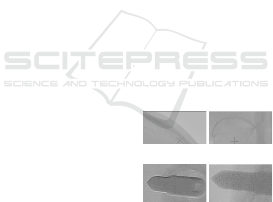
tion. This results in multiple irrelevant things being
visible. These are bones like the top of the skull and
the eye sockets (see Figure 1), the screws that hold
the stereotactic frame (see Figure 2) and the markers
on the box (see Figure 3), and possibly glue from a
previous embolization (see Figure 4). We can ignore
all effects related to the stereotactic frame but we aim
at suppressing the remaining things. Another effect
is the appearance of white borders along edges with
a strong contrast (see Figure 5). This is visible al-
ong all larger arteries. As it overlays the vessels, it
makes some vessels look disconnected. Lastly, Fi-
gure 6 shows the same artery filled with the marker
and with it flowing off a short time later. In the left
image we can discover lighter regions from inhomo-
geneous occlusion and from the second image we see
how the marker fluid mixed with the blood and the
flow creates fadings along the vessel boundaries.
The perspective as well as the patient’s position
are constant during a series. A single image has a re-
solution of 1024× 1024 with 10 bit of dynamic range.
Figure 1: Example for the skull and a eye socket remaining
visible in the DSA.
Figure 2: Examples for screws that hold the stereotactic
frame.
2.1 Time Context
For our dataset, we selected four images per DSA se-
ries, showing the same dispersion state. The images
VISAPP 2018 - International Conference on Computer Vision Theory and Applications
332
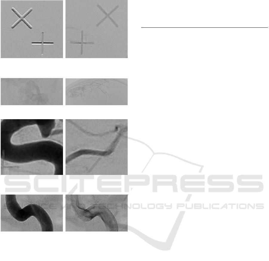
Figure 3: Examples for the markers on the box mounted to
the stereotactic frame.
Figure 4: Examples for previous glue embolizations.
Figure 5: Example for white borders along contrast rich ed-
ges.
Figure 6: Example for inhomogeneous occlusion due to the
marker flowing off from one image to the next.
are selected based on the following state descriptions:
1. the large arteries are visible
2. the complete artery tree is visible
3. the marker has flown off the largest arteries
4. no arteries, but mainly veins are visible
Arteries and veins are not connected directly in a
healthy person’s head. The transition is done via ca-
pillaries which are not visible through an x-ray. Provi-
ded the images are taken at the right moment, we have
an image right before the capillaries are active and im-
mediately afterwards. So, the usage of multiple time
points is key to distinguishing arteries and veins. Also
the separation of vessels and background is greatly
improved (see Table 2). Using multiple time points
can be described as giving the network a time context
Table 1: Probability for the occurrence of an instance of a
given class.
No. Arteries Fine
Arteries
Veins Other
1 high low very low medium
2 high high very low medium
3 low high medium medium
4 very low low high medium
to work with but we can describe the data more preci-
sely. For this, we further split the classes into arteries,
fine arteries, veins, and others. Now we can see that
we are providing multiple images with different a pri-
ori known (fuzzy) probabilities for the classes. The
mapping to the images is shown in Table 1. By choo-
sing the images based on these criteria, we enable the
network to learn to discriminate arteries better, and
effectively include a vein suppression capability.
3 NETWORK ARCHITECTURE
Our network is build based on the U-net architecture.
Now we will describe the architecture that we chose
and all changes we made to it. The complete architec-
ture is depicted in Figure 8.
3.1 Building Block
The basic building block of the network consists of
two convolutional layers followed by a pooling or an
unpooling layer, respectively. The convolutions are
all non-padded in order to prevent artifacts along the
borders due to missing input values and use 3 × 3
kernels. Thus the image size decreases by two with
every convolutional layer. Every convolution is acti-
vated with a ReLU layer. The pooling layers use max-
pooling over an 2× 2 area, effectively halving the spa-
tial dimensions. In the original U-net the number of
channels is doubled with the following convolutions,
while we are doubling the number of channels before
the max-pooling layer. This is done to respect the ge-
neral rule that bottlenecks should be prevented in the
early layers of a convolutional neural network, as sug-
gested by (C¸ ic¸ek et al., 2016; Szegedy et al., 2016).
The unpooling unit consists of multiple layers. First
the image is upsampled by the factor two, then Ronne-
berger et al., analogues to the max-pooling layer, ap-
ply a 2 × 2 convolution. The convolution also halves
the number of channels. This is followed by an acti-
vation layer. Additionally, the non-pooled output of
the layer of corresponding size from the contracting
path is now cropped to the current image size and
AngioUnet - A Convolutional Neural Network for Vessel Segmentation in Cerebral DSA Series
333
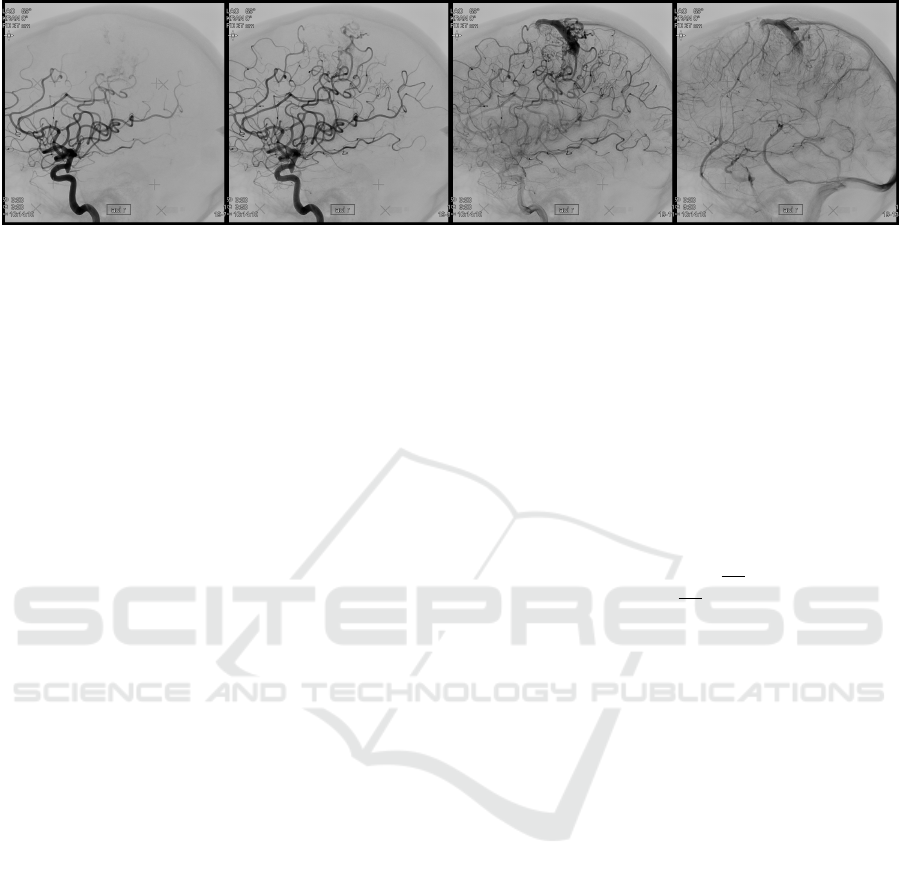
Figure 7: Example for a selection of four input images.
concatenated to the channels. This provides the ne-
cessary spatial information that was lost through the
max-pooling layers. In our network we use a 1 × 1
convolution. By visual inspection, we found that this
change results in less direction dependence of the seg-
mentation.
3.2 Tile Size
These two aforementioned variants of the building
blocks are repeated multiple times and in equal num-
ber. The U-net used four max-pooling layers, which
encoded an 572 × 572 image into 1024 channels of
the size 32 × 32. The decoded output had a size of
388 × 388. For our AngioUnet, we reduced the num-
ber of max-pooling layers to two. This decision is ba-
sed on the consideration of the receptive field as well
as the number of redundant calculations done while
training. We calculated the receptive field of the full
net to be 40 × 40. Manual evaluation of the dataset
showed that the largest vessels are usually less than 40
pixels wide. Consequently, every neuron should see
data based on both classes – vessel, and background.
While this network allows the segmentation of one
complete tile at once, there is a trade-off between re-
dundancy and peak memory load. Ronneberger et al.
also described the “overlap-tile strategy for seamless
segmentation of arbitrary large images”. This strategy
states that in order to segment an image larger than the
tile size, we extract tiles that overlap by half the num-
ber of pixels that are lost along a given dimension.
For the AngioUnet, we use 144 × 144 tiles, which are
rather small but due to the shallower architecture, the
ratio of the output size to the input size is even bet-
ter. The resulting output size is 104 × 104, thus we
extract one 144 × 144 tile every 104 pixels in every
dimension and we can use 72.2% of every tile. The
small tile size is necessary, because of text annotati-
ons in the DSA images that we excluded for training.
This way, we have to leave less tiles out that include a
part of the masked areas. It would also be possible to
change the loss function to ignore all masked pixels
but we think that this is not worth the effort, since ti-
ling and batching should not hinder the segmentation
performance.
3.3 Training
The network is trained using gradient descent. The
loss function is the cross entropy of the softmax acti-
vation of the last layer. Every epoch the learning rate
is reduced by a constant factor. The momentum is
chosen so that the initial and final learning rates α
0
and α
E
are respected:
m =
α
E
α
0
1
E−1
(1)
4 DATA AUGMENTATIONS
(Ronneberger et al., 2015) reported that data augmen-
tations were crucial for successful training of the U-
net. In our case, we use five different augmentati-
ons giving 2
3
· 3 = 24 variations of every tile. The
augmentations are mirroring along the x-axis, mirro-
ring along the y-axis, transposition, and addition and
subtraction of a bias. The first three operations pro-
vide rotation invariance by 90
◦
. One might argue that
the angiographies should be mirrored along the x-axis
only, because the images always show the vessel tree
upwards. But, we think that mirroring along the y-
axis is reasonable too, because the receptive field is
small enough and no positional information is given,
so that the network can not learn location-dependent
features but it learns to better segment thin vessels
near the bottom, which indeed run downwards.
4.1 Bias
The addition and subtraction of a bias is useful for the
given modality. A DSA image is calculated by sub-
tracting two consecutive x-ray images. This means
the gray value in the image depends on the amount
VISAPP 2018 - International Conference on Computer Vision Theory and Applications
334
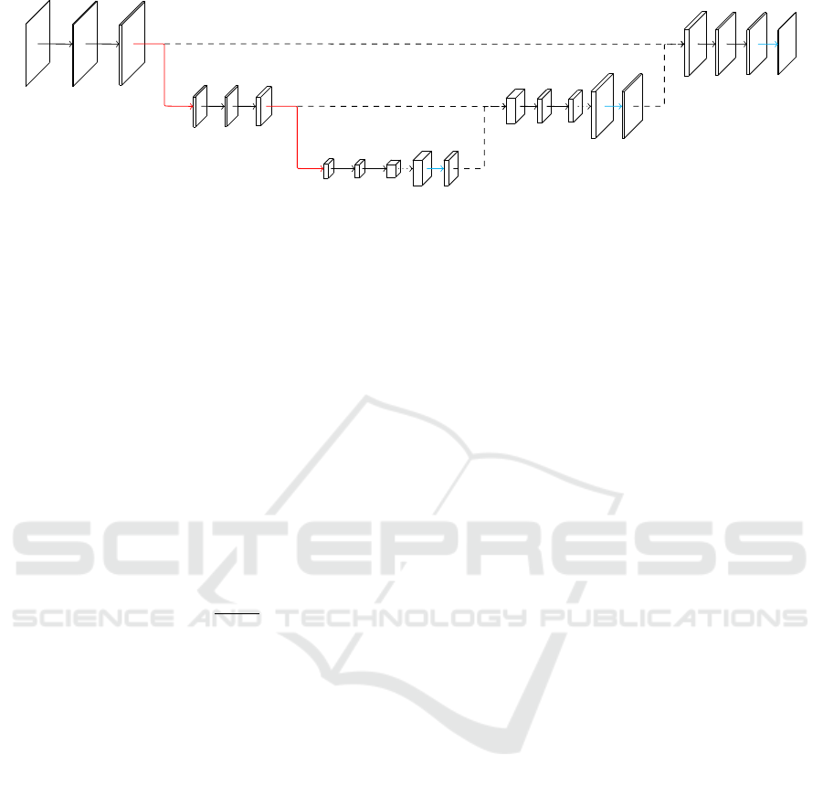
4
144×144
16
32
32
70×70
32
64
64
33×33
64
128
128
58×58
64
64
64
64
64
108×108
32
64
32
32 2
104×104
Figure 8: AngioUnet Architecture with four input images and 16 feature channels in the first convolution layer (red: max-
pooling, dotted: upsampling, cyan: 1x1 convolution, dashed: crop and concat).
of change in marker density, which itself depends on
many factors e.g. the blood flow and the quality of the
marker fluid. Introducing a constant bias is an attempt
to reduce the impact of such effects. Given an input
image I, we can describe this augmentation for every
pixel I(x, y) as follows. The simplest way is to use a
fixed bias b set to 5% of the dynamic range
b =
0.05 · 2
10
= 51 (2)
that we apply to all pixels in the inputs by addition
and clipping
I
0
(x, y) = min
max(0, I(x, y) ± b), 2
10
− b − 1
(3)
Another option is to apply a gamma correction with
γ = 0.2
I
0
(x, y) = 2
10
·
I(x, y)
2
10
1+γ
(4)
which requires no clipping and puts emphasis on the
mid range of the gray values.
4.2 Rotation Invariance
While inspecting classified images, we noticed that
the sensibility of the detection depends on the di-
rection of vessels. This is especially noticeable in
areas with synthetic shapes, e.g. text. It should be no-
ted that the effect is not symmetric along the x- or
y-axis, despite the fact that we used mirroring and ro-
tation as data augmentations. Instead, some specific
directions show a different segmentation result. Gi-
ven the small corpus for training, we think that the
segmentation should not depend on the direction, as
the network would be too specific to the dataset. We
did an experiment to make all kernels rotation sym-
metric. This can be achieved by constructing every
3 × 3 kernel from only 3 weights i.e. center w
0
, edge
w
1
and corner w
2
:
w
2
w
1
w
2
w
1
w
0
w
1
w
2
w
1
w
2
(5)
The idea behind this is that the network can not learn
to differentiate directions as a whole when every sin-
gle convolution is rotation invariant. Our tests showed
that the output is indeed independent of any direction
but at the same time the segmentation performance
is severely limited. Also this network was harder to
train i.e. it did not converge with the default learning
rate. Looking further by picking a single trained ker-
nel from the normal network, we found a filter mask
that was, in a simplified view, of the form
0 1 α
1 0 −1
0 −1 0
(6)
with α ≈ 1. This mask alone is very effective in sepa-
rating fore- and background visually. It can be noticed
that this mask is basically calculating the gradient in
a 135
◦
direction. Throughout the whole network, the
kernels are asymmetric. This suggests that the net-
work learns to encode different directions and their
combinations within the channels. Therefore, choo-
sing a smaller number of channels should lead to less
directivity. Naturally, further reduction of the number
of channels decreases performance, too.
5 EVALUATION
We evaluate all network configurations with our da-
taset. It consists of four DSA series each with four
1024 × 1024 images and a corresponding binary seg-
mentation map. The segmentation maps are hand-
labeled images. From these images, we cut 144× 144
tiles and apply all data augmentations. As described
in Section 4, the first augmentation is the addition and
subtraction of a fixed bias of 5%. Then all images are
successively transposed, mirrored along the x-axis,
and finally mirrored along the y-axis. This gives us
a total amount of 3576 tiles with four channels and a
label each. We use 80% of the tiles for training, 10%
AngioUnet - A Convolutional Neural Network for Vessel Segmentation in Cerebral DSA Series
335

for validation and 10% for testing. Additionally, we
classified an “unknown” series to confirm the genera-
lization. The training was done on a NVIDIA Quadro
K2200 within four hours.
In Table 2, the statistics for multiple configurati-
ons are presented. The standard configuration is a
network with 16 channels and a learning rate from
1· 10
−2
to 1 · 10
−6
falling exponentially over 128 epo-
chs. Configurations marked with a star needed a lo-
wer learning rate that was held constant over training
in order to be successfully trained. We gather accu-
racy, precision, and recall, and also calculate the Dice
similarity coefficient (DSC) (Dice, 1945). The DSC
is the harmonic mean of the precision and the recall:
DSC = 2 ·
precision · recall
precision + recall
(7)
As an overlap metric, it describes the total segmenta-
tion performance well, by incorporating the true posi-
tives as well as the false positives and false negatives.
It is our primary measurement when comparing dif-
ferent network configurations. The value of the cross
entry loss function is also useful to predict the achie-
vable performance earlier during training. In Figure 9
the typical convergence characteristic is shown. Ge-
0
0.1
0.2
0.3
0.4
0.5
0.6
0.7
0.8
0.9
1
0 1000 2000 3000 4000 5000
accuracy
precision
DSC
recall
cross entropy
Figure 9: Statistics of the standard configuration during the
first 5000 training steps (≈ 29 epochs). These values are
reported on the validation set.
nerally the precision starts high while the recall stays
lower. With increasing number of epochs, the re-
call improves by some percent and the precision only
decreases slightly, thus increasing the DSC slowly.
Every configuration was retrained five times. The re-
sults were averaged and the empiric standard devia-
tion was calculated. This way we can better compare
the configurations and decide if a variation is an im-
provement or due to a good random initialization.
5.1 Quantitative Evaluation
First, we will look at the different inputs. Table 2
shows the results for a network trained with the image
for state two only versus a network trained with all
four images. It is clear that the network with four
images has more information to base its decision on
and thus outperforms the single image network by
16.97%.
The next step is to compare the different vari-
ants of incorporating a bias as a data augmentation.
From Table 3 we can see that the network trained wit-
hout augmentation of the gray values performs signi-
ficantly worse. The fixed bias variant and the gamma
variant result in similar DSC values with a slight ad-
vantage for the fixed bias. It can be noted that the sta-
tistics of the network trained with a gamma correction
spread substantially more.
Finally, we tested some variations and impro-
vements proposed for different deep learning tasks:
1. Our architecture uses a 1 × 1 convolution in the
upconv operation. As described earlier, we aim at
decreasing the influence of the direction in which
a vessel is captured. When we compare the re-
sults, we can see a slight improvement in all me-
trics. This suggests that for a given number of
channels the 1 × 1 convolution is less specific
i.e. more abstract.
2. Building symmetric kernels from three weights,
as shown in Section 4.2, makes the segmentation
decision mostly invariant to the vessel direction
and reduces the number of trained parameters but
it also decreases the total performance by more
than a percent. This configuration needed a lear-
ning rate as low as 5 · 10
−4
to converge, still two
out of the five runs did not produce any positives
and thus are excluded from the statistics.
3. The number of channels in the network defines
the amount of generalization the network has to
learn by restricting the number of different featu-
res available at any given stage. Here k denotes
the number of channels after the first convolution.
In the following layers the number of channels al-
ways is a multiple of k using the scheme shown
in Figure 8. The standard configuration uses 16
channels. Halving it to eight increases the pre-
cision minimally but in total the performance is
slightly lower. Increasing k to 32 required redu-
cing the learning rate to 1 · 10
−3
and results in a
network with a DSC that is marginally lower.
5.2 Qualitative Evaluation
We can further evaluate the performance by looking
at the classification of images that are unknown to the
network. One example is given in Figure 10.
All large vessels are segmented and many finer
vessels are visible, too. One visible problem are lo-
VISAPP 2018 - International Conference on Computer Vision Theory and Applications
336
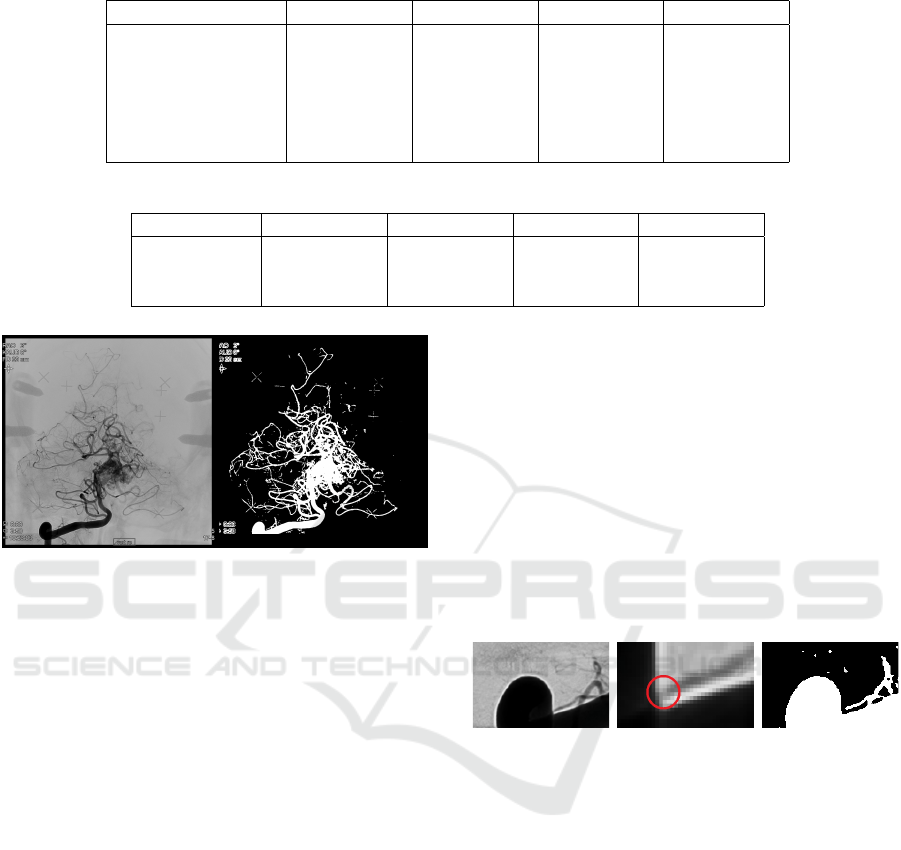
Table 2: Statistics of different configurations reported on the test set after training. All values are given in percent.
configuration accuracy precision recall DSC
standard 94.77 ± 0.08 89.41 ± 0.47 86.59 ± 0.45 87.98 ± 0.18
one image 89.13 ± 0.07 86.52 ± 0.59 60.22 ± 0.58 71.01 ± 0.27
2 × 2 upconv 94.72 ± 0.13 89.18 ± 0.98 85.96 ± 0.94 87.53 ± 0.28
k = 8 94.54 ± 0.19 89.90 ± 0.52 84.10 ± 1.56 86.90 ± 0.59
symmetric kernels* 93.99 ± 0.16 88.47 ± 3.23 83.96 ± 4.11 86.05 ± 0.67
k = 32* 94.65 ± 0.07 89.59 ± 0.64 85.76 ± 0.58 87.63 ± 0.12
Table 3: Statistics of the standard network trained with different biasing data augmentations. All values are given in percent.
configuration accuracy precision recall DSC
no bias 93.22 ± 0.20 87.23 ± 1.61 80.89 ± 1.60 83.92 ± 0.44
fixed bias 94.77 ± 0.08 89.41 ± 0.47 86.59 ± 0.45 87.98 ± 0.18
gamma 94.73 ± 0.07 88.91 ± 0.80 87.04 ± 0.96 87.96 ± 0.19
Figure 10: Example classification using the standard con-
figuration. Shown are the second input image and the seg-
mentation.
cal true positives on fine vessels that are disconnected
from the main vessel tree. These can easily be remo-
ved by an optional postprocessing step. In order to do
so, we could enumerate all components using flood
filling and only keep components whose number of
pixels is greater than a threshold.
At this point, we can look at all the requirements
we discussed earlier and see how well the network
fulfilled these based on some example patches:
1. suppression of bones (skull and eye socket)
2. suppression of glue
3. effect on screws
4. effect on stereotactic markers
5. white borders along contrast rich edges
6. inhomogeneous occlusion by the marker
The first four items have in common that the influence
on the DSA is constant over time i.e. the effect on the
gray values is the same in all input images and thus
can be easily removed by subtraction. The network
fulfilled Item 1 and Item 2 in all our experiments. For
Item 3 and Item 4 we can note that those do get seg-
mented partially, if the contrast is high (see images on
the left side of Figure 2 and Figure 3). As mentioned
before, this is not relevant for our application. The
white borders (Item 5) still pose a problem because
they disrupt the segmentation of finer vessels. An ex-
ample is shown in Figure 11. The small vessel paral-
lel to the large artery disappears inside the occlusion
of the latter in the DSA image. The artifact is additive
so that it should be possible to keep the vessel compo-
nents connected. The segmentation output shows that
the vesssel stops before the border, therefore missing
a possible connection. Item 6 seems to be no issue, so
that only in one segmentation output of the configura-
tion using one image as input an elongated hole was
visible in the largest artery.
Figure 11: Example for the white border along a large ar-
tery. The contrast of DSA images is enhanced for better
visibility.
6 CONCLUSION
We demonstrated how the U-net architecture can be
effectively applied to the segmentation of DSA series.
By basing the classification on multiple images of a
time series, we can greatly improve the segmentation
performance. For our dataset, training the network on
four images, selected for specific timepoints, gives a
DSC of 87.98% which is 16.97% better than using a
single image. As noted by (Ronneberger et al., 2015),
data augmentations proved to be helpful for impro-
ving the network’s performance while using a very
small corpus of training data. Besides rotation and
mirroring, we used biasing instead of elastic deforma-
tions so that the spatial context does not get degraded.
Overall the network produces usable segmentation re-
AngioUnet - A Convolutional Neural Network for Vessel Segmentation in Cerebral DSA Series
337

sults with the main drawback of having many isolated
true positives in regions with fine vessels.
ACKNOWLEDGEMENT
We would like to thank the Gamma Knife Krefeld
Centre for providing us with DICOM datasets and
medical expert knowledge.
REFERENCES
Badrinarayanan, V., Kendall, A., and Cipolla, R. (2015).
Segnet: A deep convolutional encoder-decoder ar-
chitecture for image segmentation. arXiv preprint
arXiv:1511.00561.
Brosch, T., Tang, L. Y., Yoo, Y., Li, D. K., Traboulsee, A.,
and Tam, R. (2016). Deep 3d convolutional encoder
networks with shortcuts for multiscale feature integra-
tion applied to multiple sclerosis lesion segmentation.
IEEE transactions on medical imaging, 35(5):1229–
1239.
C¸ ic¸ek,
¨
O., Abdulkadir, A., Lienkamp, S. S., Brox, T., and
Ronneberger, O. (2016). 3d u-net: learning dense vo-
lumetric segmentation from sparse annotation. In In-
ternational Conference on Medical Image Computing
and Computer-Assisted Intervention, pages 424–432.
Springer.
Dice, L. R. (1945). Measures of the amount of ecologic
association between species. Ecology, 26(3):297–302.
Ronneberger, O., Fischer, P., and Brox, T. (2015). U-net:
Convolutional networks for biomedical image seg-
mentation. arXiv preprint arXiv:1505.04597.
Szegedy, C., Vanhoucke, V., Ioffe, S., Shlens, J., and Wo-
jna, Z. (2016). Rethinking the inception architecture
for computer vision. In Proceedings of the IEEE Con-
ference on Computer Vision and Pattern Recognition,
pages 2818–2826.
VISAPP 2018 - International Conference on Computer Vision Theory and Applications
338
