Towards Image Colorization with Random Forests

Helge Mohn, Mark Gaebelein, Ronny H

ansch and Olaf Hellwich

Department of Computer Vision & Remote Sensing, Technische Universit

at Berlin, Germany

Keywords:

Image Colorization, Random Forests, Regression.

Abstract:

Image colorization refers to the task of assigning color values to grayscale images. While previous work is

based on either user input or very large training data sets, the proposed method is fully automatic and based on

several orders of magnitude less training data. A Random Forest variation is tailored towards the regression

task of estimating the proper color values when presented with a grayscale image patch. A simple position

prior as well as scale invariance are included in order to improve the estimation results. The proposed approach

leads to satisfying results over various colorization tasks and compares favorably with state of the art based on

convolutional networks.

1 INTRODUCTION

From the ﬁrst stable grayscale photo in history taken

in 1826 by Joseph N. Nipce, it took more than 60 ye-

ars until photography was available for the mass mar-

ket with the introduction of Kodak Nr. 1 in 1888. Co-

lor ﬁlms, however, would not been available for anot-

her 50 years. Even after the release of color ﬁlms by

Agfa and Kodak in 1936, grayscale ﬁlms remained in

common use - for speciﬁc use cases even until today

(Mulligan and Wooters, 2015).

The century, when grayscale ﬁlms have been the

only possibility to take photographs, leaves a tremen-

dous amount of pictures that would potentially bene-

ﬁt from a robust and automatic colorization method.

However, possible applications go beyond grayscale

photography and include the colorization of night vi-

sion images or the production of pseudo-color images

to emphasize certain image structures such as structu-

ral damage in X-ray images.

Assigning plausible color values to a grayscale

image is a very sophisticated task and in general an ill-

posed problem since several colors in the real world

would result in the same grayscale image. Thus, prior

knowledge needs to be included, which helps to over-

come these ambiguities. Existing work for coloriza-

tion of grayscale images can be coarsely divided ba-

sed on the source of this prior knowledge.

Color embedding is an applicational area, which

is only loosely related to colorization. Correspon-

ding methods aim at saving the chrominance infor-

mation within a given grayscale image. One example

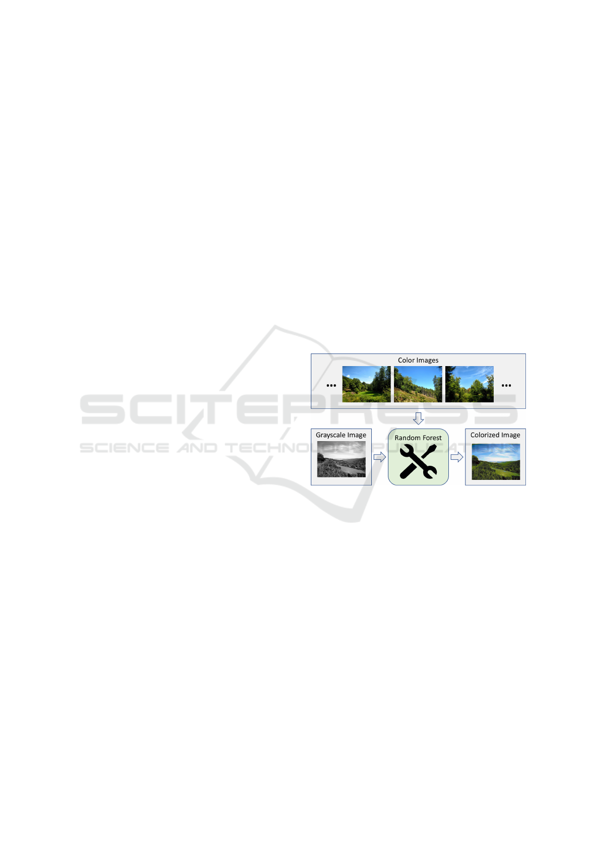
Figure 1: A Random Forest (RF) is trained with color ima-

ges that have a similar scenery as the query grayscale image.

The trained RF is able to determine a plausible color version

of a given grayscale image.

is (R. L. de Queiroz, 2006), which maps color values

to high-frequency textures of low visibility and adds

them to the grayscale image. As this process is re-

versible, it allows a color-to-grayscale conversion as

well as the “recolorization” of the obtained grayscale

image. However, it requires the availability of the cor-

responding color image so that the correct informa-

tion can be encoded into the grayscale image.

Another related ﬁeld is the color transfer between

frames of a grayscale video. Certain keyframes are

colorized by a given method, e.g. manually, and the

given color values are subsequently transferred from

one frame of the video to the next. Corresponding

methods rely on matches between the image content

which can be established either manually as in (Kar-

thikeyani et al., 2007) or automatically as in (Irony

270

Mohn, H., Gaebelein, M., Hänsch, R. and Hellwich, O.

Towards Image Colorization with Random Forests.

DOI: 10.5220/0006570002700278

In Proceedings of the 13th International Joint Conference on Computer Vision, Imaging and Computer Graphics Theory and Applications (VISIGRAPP 2018) - Volume 4: VISAPP, pages

270-278

ISBN: 978-989-758-290-5

et al., 2005). Due to the high similarity of adjacent

frames, this process provides highly accurate and re-

liable results. The question how the keyframe can be

colored is left unanswered, though.

A large group of colorization approaches involve a

human operator to exploit the vast knowledge of hu-

mans about objects in the real world. Users label a

few pixels within the image with corresponding co-

lors, which are then propagated to neighboring pixels

with similar intensity or textural patterns (A. Levin,

2004; Yatziv and Sapiro, 2006). The strength of these

approaches is certainly the user. On the one hand, hu-

mans are naturally well trained to match colors from

memory. On the other hand, colors will be selected

that are plausible on the object- or semantic level

instead of being based on low-level image informa-

tion such as texture or intensity alone. While these

approaches result in a visually pleasing color version,

the involvement of a human operator is time consu-

ming and hinders the application to a large amount of

images.

The last group consists of fully automatic appro-

aches which do not rely on any kind of manual in-

teraction. Instead, they are based on a set of trai-

ning images where additional to the grayscale images

the corresponding color information is known. These

methods derive a statistical model of the relationship

between intensity and textural patterns on the one side

and realistic colors on the other side. A recent exam-

ple is (R. Zhang, 2016) which is based on a Convoluti-

onal Network (ConvNet) which is trained on millions

of color images. The resulting network is able to co-

lorize general images and leads to visually pleasing

results.

While approaches such as (R. Zhang, 2016) are

based on millions of training images, our approach

operates with 10-20 images with the additional con-

straint that these images show a similar scene (see Fi-

gure 1). Due to the smaller amount of images, training

is very efﬁcient and can be easily tailored to speciﬁc

scenes for various applications.

It applies a Random Forest (RF, (Breiman, 2001))

for the regression task of estimating plausible co-

lor information when provided with a local grays-

cale image patch. Color information is stored as 2D

histograms over chrominance values within the CIE

L*a*b* color space. Although the RF is trained on

only a few images of a similar scene, the usage of

local image patches as well as comparatively large

histograms would lead to a large memory footprint

if naively implemented. Two solutions are proposed

to cope with this problem. First, the color histograms

at the leafs are usually sparse and can thus be sto-

red in a memory-efﬁcient manner. The second solu-

tion is based on the observation, that only tree crea-

tion needs to hold all training samples in the memory

(see Section 2.2), while tree training can be executed

on training batches (see Section 2.3). Instead of pre-

computing any kind of low-level features, the RF is

applied to the grayscale images directly. Correspon-

ding node tests compute several implicit features on

the ﬂy (as for example in (Lepetit and Fua, 2006)),

which allow memory- and time-efﬁcient processing

and are furthermore highly adaptable to the speciﬁc

colorization task. The training data is augmented with

training images at different scales to enable the forest

to map scaled textures to the correct colors. Obser-

ved color values are rebalanced similar to (R. Zhang,

2016) to account for the fact that pastel colors occur

more frequently than saturated colors.

The contribution of the proposed method is there-

fore ﬁve-fold:

• Decoupling tree creation and tree training to make

full use of a large amount of training samples du-

ring the estimation of the target variable.

• Implicit feature learning makes the computation

of predeﬁned features obsolete.

• A sparse representation of the target variables le-

ads to memory-efﬁcient RFs.

• Data augmentation increases the robustness of the

colorization regarding scale.

• Color rebalancing leads to realistically saturated

colors.

2 COLORIZATION ALGORITHM

2.1 Preprocessing

The proposed colorization method is based on a RF

(see Sections 2.2-2.4) as regression method. As su-

pervised approach, it relies on training data which -

additionally to the grayscale images - provides the

corresponding color information. While ground truth

data is difﬁcult to obtain in many other supervised ma-

chine learning problems such as semantic segmenta-

tion, it basically comes for free for colorization tasks.

Any kind of color image can be transformed into a

grayscale version where the latter is used as training

data and the former as reference image. The propo-

sed method uses the CIE L*a*b* color space to per-

form regression, since it decouples luminance from

color information. Thus, training images are conver-

ted from RGB to CIE L*a*b*, where the luminance

L* is used as training input and the a*b* components

as target variable. During prediction, the luminance

Towards Image Colorization with Random Forests

271

is provided by the query image itself, which is then

fused by the estimated chrominance information to

obtain a color image.

During application, the RF aims at matching tex-

tural patterns in the query image to patterns observed

during training. However, images of similar scenes

and objects can differ largely in brightness and con-

trast due to different lighting conditions. In order to

normalize for lighting changes, histogram equaliza-

tion is performed as preprocessing step, which allows

a better comparability of different image patches.

Another change that commonly appears in opti-

cal imagery of close-range objects is a variation in

scale: While textural properties of an object might

differ greatly depending on the distance the image is

acquired, the color stays more or less constant. A cor-

rect colorization result can only be expected, if the

scale of the object within the query image is similar

to the scale within the training images. That is why

the training data is augmented with differently scaled

versions of the training images in order to achieve a

certain scale invariance.

2.2 Creation of a Random Forest

A RF is a set of binary decision trees, where each tree

is a hierarchical structure of split- and leaf-nodes. All

trees are created independently from each other and

should be as diverse as possible in order to beneﬁt

from averaging their results during prediction. Diver-

sity is usually achieved by introducing randomization

processes during tree creation. A ﬁrst source of rand-

omization is bagging, i.e. creating individual training

sets for each tree by randomly sampling data from the

training set.

During tree creation, split nodes are subsequently

added to a tree starting by the root node. Every split

node partitions the data that was propagated to this

node based on a simple binary test Ψ. Depending on

the outcome of this test, the corresponding subsets are

propagated further to the left or right child node. The

performance of each tree and thus of the whole fo-

rest depends strongly on the deﬁnition and selection

of reasonable node tests. Vanilla RF implementati-

ons usually simply split along one randomly selected

feature dimension, which in our application scenario

corresponds to test whether the luminance L of a cer-

tain pixel (x + ∆x, y + ∆y) within the patch at (x, y) is

higher or lower than a threshold T . Equation 1 shows

this ﬁrst luminance feature (Ψ

), which basically de-

termines whether a pixel belongs to a bright or a dark

object. This work additionally applies node test va-

riants that are more tailored towards the analysis of

images (as for example proposed in (Lepetit and Fua,

Figure 2: From left to right: Part of a grayscale image; Ex-

ample patches taken from marked pixel positions; Lumi-

nance feature Ψ

; Luminance difference feature Ψ

. The

two rows show a homogeneous patch at the top and a textu-

red patch at the bottom.

2006)). Equation 2 shows a second luminance feature

which compares the luminance difference of two

pixels (x +∆x

, y +∆y

), i ∈ {1, 2} located in a patch at

(x, y) to a threshold T . This feature is an approxima-

tion of the local gradient and thus analyses the local

texture. Figure 2 visualizes these two features.

: L(x + ∆x, y + ∆y) ≥ T (1)

: L(x + ∆x

, y + ∆y

) − L(x + ∆x

, y + ∆y

) ≥ T

(2)

A second group of node tests aims at including a

prior model on the positions that different colors take

within an image. Depending on the application sce-

nario, i.e. the nature of the query image, some colors

are more likely to occur at certain image positions.

Simple examples are landscape images, which often

show blue pixels at the top (i.e. the sky) or portraits

that show pixels of skin color rather in the center.

Three different node tests are used to enable the

RF to learn the color prior from the training data. The

ﬁrst variant tests whether the pixel coordinates of a

patch are within a circular area, whose position and

size are randomly determined. The other two variants

simply split either on the x- or on the y-coordinate of

the patch position (very similar to test type Ψ

) and

thus divide the image into axis-aligned blocks.

Nearly all of the used node tests involve the com-

parison of a scalar value (either luminance or pixel

coordinate) with a threshold. There are many ways to

deﬁne this threshold ranging from random sampling

to a completely optimized selection. We deﬁne the

threshold as the median of the projected values as this

splits the data into two equally large parts (if possi-

ble). This leads to trees that are most balanced. Thus,

they apply a maximum amount of node tests to the

data and achieve a ﬁne-grained partition of the feature

space. However, this threshold deﬁnition depends on

the data only and is independent of the reference data.

VISAPP 2018 - International Conference on Computer Vision Theory and Applications

272

In order to optimize the node tests with respect to

the target variable, each newly created split node ge-

nerates multiple different test candidates during tree

creation. These different test instances are created by

randomly sampling test parameters, e.g. which of the

ﬁve different test types is applied, which pixel positi-

ons are to be used, etc. Each of these tests splits the

local data into two subsets. Based on this split, the

drop of impurity (Eq. 3) is computed which is based

on the Gini index (Eq. 4).

Γ = I

node

− (P

le f t

· I

le f t

+ P

right

· I

right

) (3)

= 1 −

∑

a,b

(a, b)

(4)

where p

is the distribution of colors represented as

2D histogram over the a*b* values of the CIE L*a*b*

color space at node n.

The test leading to the split with the largest drop

of impurity is selected and the samples are propagated

to the child nodes accordingly.

The recursive splitting stops, if one of the follo-

wing criteria is met:

• The maximum tree height is reached.

• The minimum number of samples within a node

falls below a threshold.

• The largest drop of impurity of all generated split

candidates is below a threshold (i.e. close to zero).

2.3 Training of a Random Forest

As colorization is an inherently ill-posed problem it

beneﬁts from the virtually unlimited amount of trai-

ning data. The creation of the random decision trees,

however, relies on the availability of all data sam-

ples in order to perform node test optimization (see

Section 2.2). Thus, only a certain fraction of available

training samples is used to deﬁne the tree structure.

Once the trees are created, they have to be trained, i.e.

an estimate of the target variable has to be assigned

to the corresponding leaf nodes. This process does

not require all samples to be present at once. Thus, to

train the trees all samples from all training images are

used.

Training patches are propagated through the tree

based on the node tests as deﬁned during tree creation.

Once a patch reaches a leaf node, it is used to update

the estimate of the target variable, i.e. the correspon-

ding color. To this purpose the color information is

quantized and stored in two-dimensional histograms

representing the local posterior of the a*b* part of the

CIE L*a*b* color space. Due to the nature of the de-

cision trees, these histograms tend to be very sparse

Figure 3: Histogram normalization: Left: Ground truth

image (a green tomato); Right: Colorization results. Wit-

hout normalization (top) the tip of the tomato is falsely co-

lored in green, while it is correctly colored brownish if all

histograms are normalized according to the chrominance

occurrence in the training data (bottom).

and can thus be saved in an efﬁcient manner in order

to minimize the memory footprint of the trees.

At the end of the training process all histo-

grams are normalized according to the hue occurrence

within the training data. This class rebalancing is a

typical processing step to ensure that classes that are

underrepresented within the training data are treated

with similar importance as frequent classes. This is

especially important in colorization tasks, since rat-

her weak colors appear signiﬁcantly more often than

strongly saturated colors. Colors with a high occur-

rence in the training images would then dominate nu-

merous hue histograms.

Figure 3 shows an input image on the left. The top

of the right side shows a detail of the colorization re-

sult without normalization after the training process,

while the bottom right illustrates the colorization re-

sult with normalization. In this example green is the

dominant color which clearly dominates brown. Wit-

hout proper normalization the brown tip of the tomato

is falsely colorized in green. After performing a nor-

malization the tomato point is correctly colorized in

brown.

2.4 RF Application

During prediction, patches around all pixels of the

query image are propagated through the trees in the

same way as during tree training. A patch x will re-

ach exactly one leaf n

in each individual tree t. Let

(a, b|x) be the a*b* histogram of the particular leaf

in tree t that had been reached by patch x. The

a*b*-histograms of these leafs are averaged and the

maximal value of the resulting histogram is assigned

as chrominance estimate ˆa*

b* to the corresponding

pixel:

Towards Image Colorization with Random Forests

273

ˆa

∗

= argmax

a,b

p(a, b|x) (5)

p(a, b|x) =

∑

t=1

(a, b|x) (6)

The estimated ˆa*

b*-values together with the

grayscale value of the query image provide the com-

plete CIE L*a*b*-vector which is then converted to

the RGB color space and saved at the corresponding

image position.

3 EVALUATION

3.1 Data

The proposed method assumes a small database of

images similar to the query image (see Figure 1). The

difﬁculty of the colorization task depends on the con-

tent of the query images and how well their statistics

match the statistics of the training data. These two

factors are somewhat connected: If scenes have a li-

mited color variation and a clear relationship between

texture and color, it is more likely to sufﬁciently re-

present them with a few training images. If scene

content is diverse and similar textures are colored dif-

ferently, the training data might not sufﬁce to extract

all necessary information and even if, the estimated

mapping will be ambiguous. In order to evaluate the

performance without having a selection bias towards

too easy (or too hard) image types, we collected data

for ten different and diverse categories, namely Be-

ach (see for example Figure 10), Sanssouci, Redbrick-

House, GarbageCan, PolarLight, Airport, Train, Gra-

pes (see for example Figure 8), and Forest (see for

example Figure 12). These categories include man-

made as well as natural objects, homogeneous as well

as strongly textured regions, and cover a wide range

of color distributions.

3.2 Random Forest Statistics

The colorization results depend solely on the perfor-

mance of the applied Random Forest since no other

type of processing (e.g. label smoothing as post pro-

cessing) is involved.

That is why this section brieﬂy analyzes an exam-

ple instance of a Random Forest that was trained on

images of the category Sanssouci with an image pa-

tch size of 5 × 5 pixel. It consists of four trees that

have been grown until maximal height. A node nee-

ded to contain at least 10 samples to continue split-

ting. In this case, 150 possible split candidates are

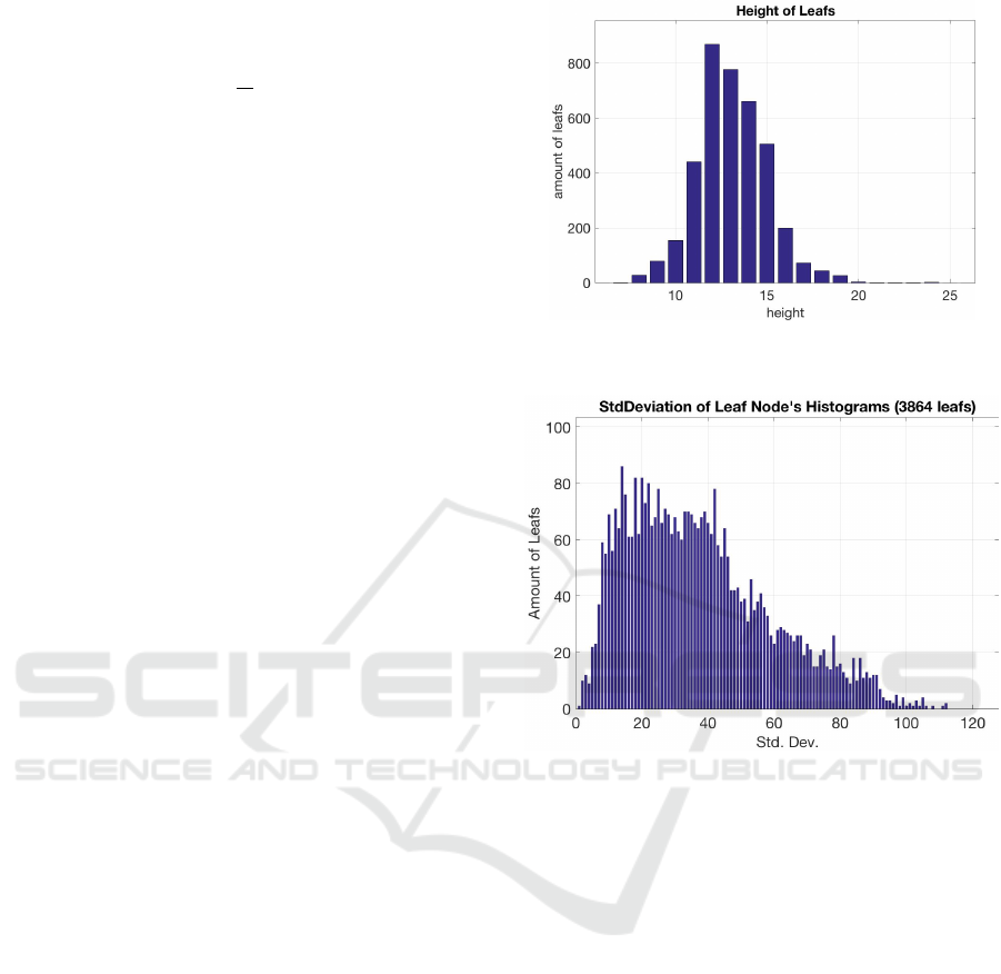
Figure 4: Amount of leafs at different tree levels within a

tree of the forest.

Figure 5: Amount of leafs with different levels of pureness

measured as average sample distance to sample mean.

created randomly and evaluated based on the drop of

impurity (see Equation 3). If the drop of impurity of

the best split was below 10

−4

or other stopping cri-

teria became valid, the recursive partitioning stopped.

In this case, a leaf node is created containing a 2D

histogram over possible a*b* values discretized into

a 32 × 32 grid.

Figure 4 shows the number of leafs existing at a

speciﬁc tree height within a tree of the forest. The

longest path within the forest only reached a height

of 24. Most paths end before height 16, which shows

that the trees are fully grown. Increasing the maximal

tree height will not change the tree topology unless

they are induced with a larger set of training samples.

Each internal node within a tree aims at dividing

the data in a way such that the corresponding child

nodes are as “pure” as possible, i.e. contain samples

mostly having similar colors. One way to measure the

“pureness” of a node in a regression tree is to compute

the average distance of the samples to their mean va-

lue. Figure 5 shows the number of leafs with different

“pureness” levels. As can be seen, most of the leafs

VISAPP 2018 - International Conference on Computer Vision Theory and Applications

274

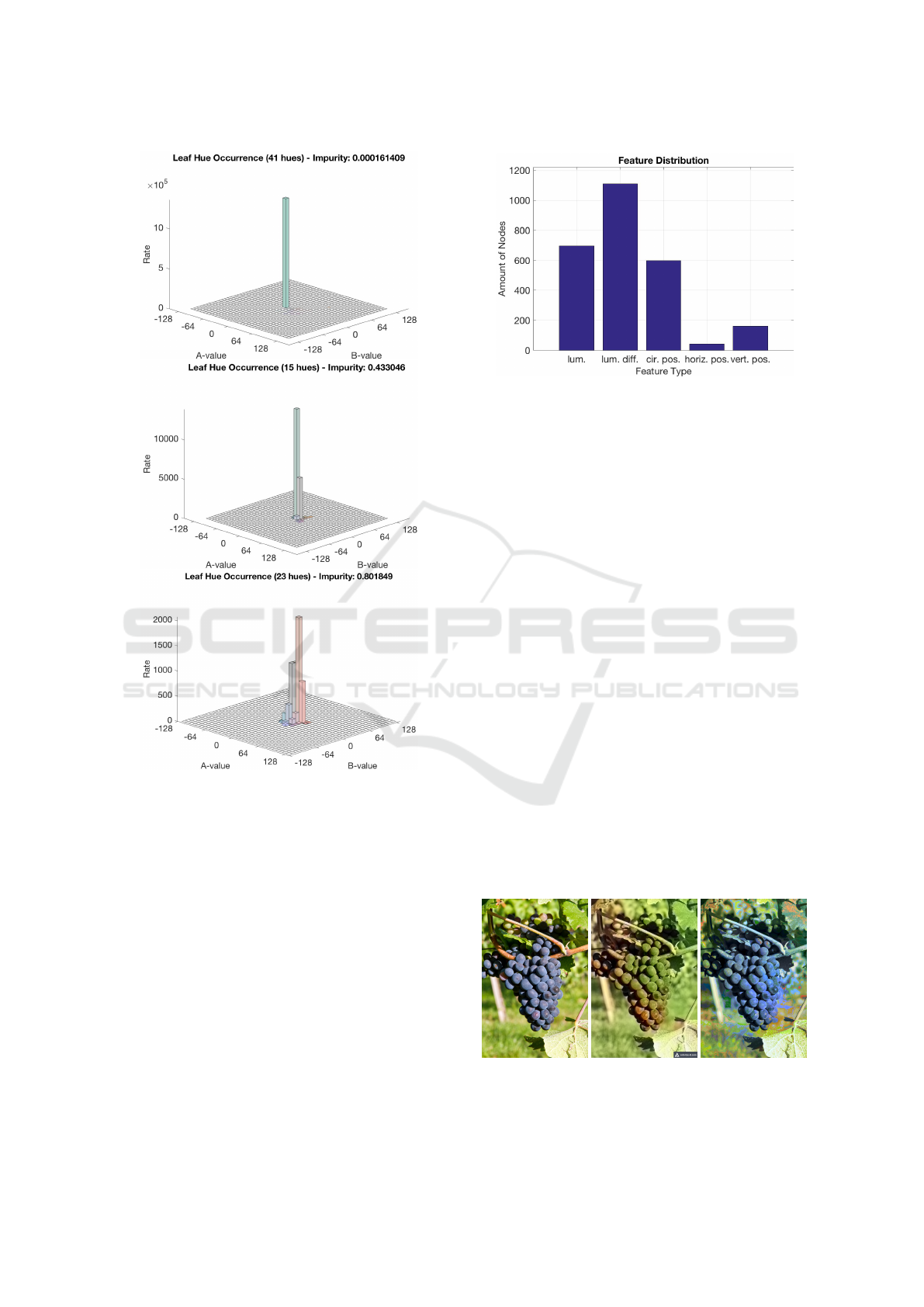
Figure 6: Hue histograms of different leaf examples.

contain samples that concentrate within a small re-

gion around the mean value (e.g. less than 40), while

only a few leafs have a very diverse set of colors (e.g.

average distance more than 80).

Figure 6 shows the estimated histograms of three

different leaf examples with different impurities (see

Equation 4). As can be seen, even for leafs with high

impurity the colors have been well clustered by the

forest and stay within close proximity to each other.

Instead of acting as a pure black-box system,

Random Forests allow some insights into their deci-

sion making process. One example is the frequency

how often certain node tests have been performed. Fi-

gure 7 shows the selection frequency of the implicitly

calculated features (see Section 2.2). The luminance

difference of pixels inside a patch (test type Ψ

) has

been used most often, followed by the luminance va-

Figure 7: Frequency how often a certain node test is perfor-

med within a tree of the RF.

lue itself (test type Ψ

). While the latter distinguishes

between dark and bright patches, the former analy-

ses the local texture by approximating the luminance

gradient. As spatial prior information the circular re-

gion prior (see Section 2.2) is preferred over the x-y-

position.

3.3 Results

Image colorization is an ill-posed problem: The same

texture might have very different colors. One example

is the color of the hair of a person, which can - taken

artiﬁcial hair colors into account - be practically any-

thing despite having very similar textures. On the ot-

her hand, the goal of image colorization is often not to

assign the “correct” color (i.e. the color the object had

when the grayscale picture was taken), but to assign

a realistic color (i.e. the color objects of this category

usually have). Thus, achieving a visually pleasing re-

sult is often more important than a “correct” result or

- in other words - a “wrong” result can still be accep-

table for a human observer.

This is illustrated in Figure 8, which shows the co-

lorization result of the proposed method on the right

and the result of the reference method (R. Zhang,

Figure 8: Rather than assigning a correct color, assigning

a realistic color is important. From left to right: Original

image; Colorized by (R. Zhang, 2016); Colorized by pro-

posed method.

Towards Image Colorization with Random Forests

275

2016) in the center. Both results are not correct

in a numerical sense: The proposed method co-

lors the blurry background in blueish colors giving

it a ﬂowerbed-like look, while it is supposed to be

green. The reference method colors the grapes in a

greenish-brownish color. Nevertheless, both results

look equally plausible and visually pleasing.

However, the subjective quality of a colorization

result is hard to measure. Thus, we rely on objective

measurements that are based on comparing the esti-

mated color image to the ground truth. In particular,

we state the accuracy A

(E) of the estimation E with

respect to a reference image R as

(E) =

∑

(x,y)∈E

acc

(E(x, y), R(x, y)) (7)

acc

(e, r) =







1 if





∗

− r

∗

− r

∗





< θ

0 otherwise.

(8)

This measure simply counts how many pixels have a

color difference smaller than a certain threshold θ.

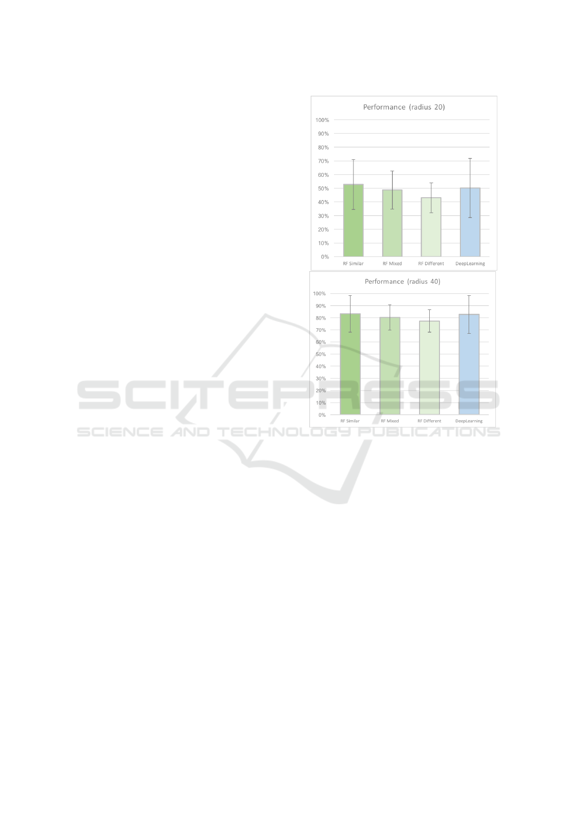
Even within a category, the image content can

vary largely, e.g. day vs. night images of a building

or summer vs. winter images of a landscape. That is

why the training images within a category are divided

into three groups: Similar to the query, dissimilar to

the query, and mixed. On each of these three groups

a separate Random Forest is trained and evaluated on

the common query images.

The performance is shown in Figure 9 for a dis-

tance threshold of 20 and 40, respectively. The top

of Figure 9 shows that on average more than 50% of

all pixels of all query images in all categories are cor-

rectly classiﬁed (i.e. have a color difference smaller

than 20 to the reference image), if the training data-

base is similar to the query. If the training database

is dissimilar to the query, this value drops by roughly

10%.

The last column shows the performance of the re-

ference method proposed by (R. Zhang, 2016). It

should be noted that this method is based on training

a deep convolutional network on millions of images.

This tremendous effort during training allows the net-

work to colorize general images during prediction.

Our method, on the other side, is trained on a rather

small database of training images which have to be

of the same category as the query image. The results

of the deep network are slightly worse than the per-

formance of the Random Forest if the training images

are similar to the query. Thus, the proposed frame-

work presents an alternative to the deep network in

the case where training on many images is either not

possible or not desired.

The bottom of Figure 9 shows the same statistics

for a threshold of 40. The accuracy of all variants go

Figure 9: Accuracy A

(Top: θ = 20; Bottom: θ = 40; see

Equation 7) of the proposed approach (ﬁrst three columns)

trained on different datasets as well as of the reference met-

hod (last column).

up to roughly 80% indicating that additional 30% of

pixels are classiﬁed with a similar color to the origi-

nal.

Figure 10 and Figure 12 show two more coloriza-

tion results additionally to those in Figure 8. The top

row shows the original image on the left and the cor-

responding grayscale image on the right. The second

row shows the colorization result obtained by the pro-

posed method with the corresponding error map on

the right where black means a correct colorization and

white corresponds to the maximum Euclidean dis-

tance between estimated and reference chrominance.

The third row shows the colorization result obtained

by the reference method (R. Zhang, 2016) together

with the corresponding error map.

Figure 11 shows the images that have been used

to train the Random Forest that has colored the image

in Figure 10. While showing a very similar scene,

the actual image content is general enough (given

VISAPP 2018 - International Conference on Computer Vision Theory and Applications

276

Figure 10: Results of example image from the Beach ca-

tegory; The top row shows the original color image on the

left as well as the grayscale version on the right. The second

and third row show on the left the colorization results of the

proposed and reference method, respectively, as well as the

corresponding error maps on the right.

Figure 11: Training images for result in Figure 10.

the category) to easily ﬁnd colored examples. The

proposed approach achieves an accuracy of A

53.63% while the reference method obtained A

50.03% The canopy of the palm tree is very well re-

constructed by the proposed method while it stays

greyish-brownish in the result of the reference met-

hod. The result of the deep learning approach has less

saturation in general but looks slightly more realistic.

The stem of the tree is not very well reconstructed by

Figure 12: Results of example image from the Forest ca-

tegory; The top row shows the original color image on the

left as well as the grayscale version on the right. The second

and third row show on the left the colorization results of the

proposed and the reference method, respectively, as well as

the corresponding error maps on the right.

both methods.

Figure 12 shows the results of the colorization of

a forest image. While the deep learning approach

reaches a colorization correctness of A

= 91.98%,

the proposed method achieves a slightly worse accu-

racy of A

= 90.04%. Although the proposed method

achieves a higher accuracy over the grass area within

the image, both colorization results are very plausible.

4 CONCLUSIONS

Instead of aiming at a general purpose colorization

tool, the proposed method focuses on the use case

where a small but speciﬁc database of training ima-

ges is available for query images of a certain category.

This keeps training time at a minimum and allows to

lessen ambiguities, which otherwise frequently occur

in colorization tasks.

The proposed method is based on a Random Fo-

rest, which analyses the local structure of a grayscale

patch and employs a spatial color prior model, which

is learnt from training data. The color information

is saved within the terminal nodes as 2D histograms

over a*b* values of the CIE L*a*b* color space.

Experiments are conducted over a range of dif-

ferent image categories including several man-made

and natural scenes. The results indicate that the pro-

Towards Image Colorization with Random Forests

277

posed method is successfully able to colorize grays-

cale images if a suitable database of training images

is available. The obtained colorization results are on

par with a reference method which is based on a deep

convolutional network trained on millions of images

and used for general colorization tasks.

Future work will focus on weakening the require-

ments on the speciﬁcity of the training images. More

diverse images allow in principle the colorization of a

broader range of query images on the cost of a more

time- and memory-expensive training phase. This re-

quires the deployment of more and deeper trees.

A further direction is the post-processing of the

obtained raw colors. A conditional random ﬁeld de-

ﬁned over the image space would allow to achieve a

local color consistency as well as taking more global

image characteristics into account.

REFERENCES

A. Levin, D. Lischinski, Y. W. (2004). Colorization using

optimization. ACM Transactions on Graphics (TOG)

- Proceedings of ACM SIGGRAPH.

Breiman, L. (2001). Random forests. Statistics Department

University of California Berkeley, CA 94720.

Irony, R., Cohen-Or, D., and Lischinski, D. (2005). Colo-

rization by example. In Eurographics Symposium on

Rendering.

Karthikeyani, V., Duraiswamy, D. K., and Kamalakkannan,

P. (2007). Conversion of gray-scale image to color

image with and without texture synthesis. Internatio-

nal Journal of Computer Science and Network Secu-

rity, 7(4).

Lepetit, V. and Fua, P. (2006). Keypoint recognition using

randomized trees. IEEE Transactions on Pattern Ana-

lysis and Machine Intelligence, 28(9):1465–1479.

Mulligan, T. and Wooters, D. (2015). Geschichte der Foto-

graﬁe. Von 1839 bis heute. TASCHEN.

R. L. de Queiroz, K. M. B. (2006). Color to gray and back:

Color embedding into textured gray images. IEEE

Transactions on Image Processing, 15(6).

R. Zhang, P. Isola, A. A. E. (2016). Colorful image colori-

zation. In ECCV 2016, volume III, pages 649–666.

Yatziv, L. and Sapiro, G. (2006). Fast image and video co-

lorization using chrominance blending. IEEE Tran-

sactions on Image Processing, 15(5).

VISAPP 2018 - International Conference on Computer Vision Theory and Applications

278