Interactive Hyper Spectral Image Rendering on GPU
Romain Hoarau
1
, Eric Coiro
1
, Sébastien Thon
2
and Romain Raffin
2
1
Onera - The French Aerospace Lab, Salon-de-Provence, F-13661, France
2
Aix Marseille University, Toulon University, CNRS, ENSAM, LSIS, Marseille, France
Keywords:
Spectral Image Rendering, Global Illumination, GPU Computing, Predictive Rendering.
Abstract:
In this paper, we describe a framework focused on spectral images rendering. The rendering of a such image
leads us to three major issues: the computation time, the footprint of the spectral image, and the memory
consumption of the algorithm. The computation time can be drastically reduced by the use of GPUs, however,
their memory capacity and bandwidth (compared to their compute power) are limited. When the spectral
dimension of the image will raise, the straightforward approach of the Path Tracing will lead us to high
memory consumption and latency problems. To overcome these problems, we propose the DPEPT (Deferred
Path Evaluation Path Tracing) which consists in decoupling the path evaluation from the path generation. This
technique reduces the memory latency and consumption of the Path Tracing. It allows us to use an efficient
wavelength samples batches parallelization pattern to optimize the path evaluation step and outperforms the
straightforward approach when the spectral resolution of the simulated image increases.
1 INTRODUCTION
Aircraft detection in the IR (Infrared) and Visible
bands is an active research field in the aerospace com-
munity. Dimensioning the sensors for this purpose re-
quires the spectral radiance of a scene at their input,
that can be expensive and difficult to obtain by air-
borne measurement campaigns. A fast and accurate
simulation (fig. 1) of these data is thus needed.
(a) 100 channels in the SWIR
range.
(b) 400 channels in the
Visible range.
Figure 1: The spectral output of a pixel (red point on both
images) and its displayable color can be visualized at the
same time.
In the IR range, local illumination methods (e.g.
(Whitted, 1979)) are used to simulate the light trans-
port in most cases for former aircraft generation or
supersonic flight where IR signature is overwhelmed
by the radiation of hot parts. Nevertheless these met-
hods have proved to be insufficient since the new ge-
neration of aircrafts relies on their shape (e.g. curved
nozzle) to hide their hot parts to improve their stealth
characteristic. Hereafter, the inter reflexions have to
be taken into account. For the aircraft IR signature si-
mulation, the aerospace community has begun to use
global illumination methods (e.g. (Coiro, 2012)). The
typical scene is an aircraft surrounded by an environ-
ment map which contains the radiation of the sky and
the ground. The scene can also contain the volume of
the atmosphere and the plume (aircraft exhaust com-
bustion gases).
The spectral output of this simulation can be sto-
red in channels of a spectral image. A channel is not a
wavelength but the integration of the spectral radiance
over a spectral interval. The spectral resolution of this
image has to be very high for the following reasons:
• The evolution of technology leads us to explore
new concepts of sensors from 380 to 20,000 nm,
at high resolution (a few nm of accuracy in visible,
and larger in IR).
• The gases of the atmosphere (fig. 2) and the air-
craft’s plume can have very spiky absorption and
emission spectrum.
Hoarau, R., Coiro, E., Thon, S. and Raffin, R.
Interactive Hyper Spectral Image Rendering on GPU.
DOI: 10.5220/0006549800710080
In Proceedings of the 13th International Joint Conference on Computer Vision, Imaging and Computer Graphics Theory and Applications (VISIGRAPP 2018) - Volume 1: GRAPP, pages
71-80
ISBN: 978-989-758-287-5
Copyright © 2018 by SCITEPRESS – Science and Technology Publications, Lda. All rights reserved
71

Figure 2: The absorption spectrum of the atmosphere (Ro-
hde, 2007).
The rendering of a such spectral image will lead
us to three major issues:
• The computation time: Each channel must be pro-
cessed.
• The footprint of the spectral image: 4 bytes per
channel per pixel.
• The memory consumption of the algorithm: For
instance, the Path Tracing (Kajiya, 1986) needs
to consume 8 bytes at least (to accumulate the
spectral radiance and the path throughput) per wa-
velength sample per path.
The computation time can be drastically reduced
by the use of GPUs, but their memory capacity and
bandwidth are limited. The straightforward appro-
ach of the Path Tracing would be to evaluate at each
bounce the path extension for each wavelength sam-
ple.
To be efficient, a path has to be reused by at le-
ast one wavelength sample per channel. When the
number of channels will raise, the wavelength sam-
ple states won’t be able to fit into the registers or the
local memory. Therefore, they would have to be sto-
red in the global memory which would imply to high
memory consumption and latency problems.
To overcome these problems, we propose the
DPEPT (Deferred Path Evaluation Path Tracing)
which consists in decoupling the path evaluation from
the path generation. At each bounce, the bare mi-
nimum information is stored in a path vertex. Once
the path is completed, the wavelength sample of each
channel is evaluated. Since the path vertices are sa-
ved, the channels can be evaluated per batch to re-
duce the memory consumption. The state of this batch
can be stored in the local memory to reduce latency.
This method allows us to optimize the path evaluation
and outperforms the straightforward approach when
the spectral resolution of the simulated image raises.
Our approach enables to render efficiently multi, hy-
per and even ultra (more than 1,000 channels) spectral
image.
Our research are beneficial to some Computer
Graphics fields such as the predictive rendering and
the colorimetric validation. The main contributions
of this article are:
• A framework to render a spectral image composed
with K number of channels (section 3).
• A suitable path tracing method (DPEPT) to ren-
der a high spectral dimension image on GPU
(section 5.1).
• An efficient wavelength parallelization pattern of
the path evaluation step (section 5.2).
2 PREVIOUS WORKS
2.1 GPU Implementation of the Path
Tracing
The Path Tracing (Kajiya, 1986) is the simplest global
illumination algorithm. Its implementation on GPU
was first studied by (Purcell et al., 2002) which pro-
posed a multi pass approach due to the lack of pro-
grammability of the early hardware.
One of the main problems at this time was the va-
rious lengths of the path which implied an inefficient
workload and code divergence. A few threads pro-
cess the long paths while other threads are idle. To
solve this problem, (Novák et al., 2010) introduced
the Regenerative Path Tracing which decouples path
from pixel by using the thread persistent technique.
If a thread is idle it generates a new path instead of
waiting.
To improve the Regenerative Path Tracing, (Ant-
werpen, 2011) proposed the Streaming Path Tracing
which compacts the regenerated threads to increase
their coherence for their primary closest intersection
tests.
Later, (Laine et al., 2013) highlighted the regis-
ter pressure problem of the mega kernel approach
(one single kernel devoted to the algorithm), especi-
ally when complex materials are used. They intro-
duced the Wavefront Path Tracing, which splits the
algorithm in different kernels. In order to reduce the
register spilling and to improve the coherence, a ker-
nel was dedicated to each material. This implementa-
tion showed a performance gain with scene made of
complex materials. However, for a scene containing
simple materials, the sorting step (to dispatch the wor-
kload to each kernel) and the kernel launching over-
head neutralized the performance gain.
GRAPP 2018 - International Conference on Computer Graphics Theory and Applications
72

(Davidovi
ˇ
c et al., 2014) made an exhaustive GPU
implementation survey of the Path Tracing. They pro-
posed new approaches and benchmarked the different
implementations. The Multi Kernel Streaming Path
Tracing was the most performance portable imple-
mentation.
2.2 Spectral Rendering
To simulate correctly the light transport, Spectral
Rendering is mandatory. Within the computer
graphics community, Spectral Rendering is used to
make colorimetry validation and predictive rendering.
The simplest way to do spectral rendering consists
in carrying one wavelength per path. However, this
approach proves to be inefficient because a path is of-
ten valid for more than one wavelength. (Evans and
McCool, 1999) proposed to reuse a path for a clus-
ter of wavelengths sampled by the lights of the scene.
To handle the refractions (one ingoing and outgoing
direction valid for only one wavelength), the authors
proposed three strategies:
• Degradation: A wavelength is chosen to conti-
nue the path. The other wavelengths are degraded
(their propagation are stopped), which increases
the variance.
• Splitting: The path is split for each wavelength.
This strategy is not easy to implement and it is
time consuming.
• Deferral: A path is generated for one wavelength.
If no refraction occured, the path is reused to com-
pute the other wavelengths.
(Radziszewski et al., 2009) improved this techni-
que by introducing a spectral sampling during the
path generation. In order to reduce the variance, the
authors suggested to use a MIS (Multi Importance
Sampling) (Veach and Guibas, 1995) to take into ac-
count the different probability density functions of the
wavelength carried by a path.
(Wilkie et al., 2014) clarified the use of multiple
wavelengths per path and the MIS method. They pro-
posed a simple but optimized approach. The cluster
of wavelengths was generated by one wavelength (na-
med “hero wavelength” by the authors) by applying a
regular offset in order to cover the visible range.
3 SPECTRAL IMAGE
RENDERING FRAMEWORK
3.1 Why Can’t We Use the Previous
Spectral Rendering Works?
The goal of the Spectral Rendering methods in the
Computer Graphics community is to compute the
tristimulus XYZ. This triplet can be seen as three
overlapping channels over the Visible range which in-
tegrate the same wavelength samples with different
sensor response curve (CIE XYZ curves). These met-
hods don’t match our objectives since:
• The spectral output of each channel have to be
conserved without the integration of a sensor re-
sponse curve (e.g. CIE XYZ curves).
• The channels don’t always overlap, therefore they
can’t share the wavelength samples. The spectral
domain of the light transport equation has also to
be discretized.
• The channel intervals are not always adjacent and
uniformly sized. Therefore this dismisses the
usage of a regular offset method (Wilkie et al.,
2014) to generate a path wavelength cluster.
3.2 The Inputs and Output of the
Simulation
The inputs of simulation are spectral data (reflectance,
complex index of refraction, ...). They can be stored
as a tabulated spectrum, but the bounds retrieval of a
query (wavelength sample) to compute the interpola-
ted value requires the use of a binary search. At the
moment, we use regular spaced spectrum which gives
us a good performance since we can easily retrieve
the bounds. The number of sample of each spectrum
is entirely dynamic which gives us a good accuracy if
needed.
3.3 The Spectral Output Data Structure
The spectral output of the simulation must be stored in
a suitable data structure. An efficient and robust data
structure for these data is an open problem, further
research has to be done. The most straightforward
approach is the use of a spectral image composed with
K numbers of channels, nevertheless it is memory-
wise (3d image) and computation-wise (each channel
needs to be processed) inefficient.
As described previously, a channel is not a wa-
velength but the integration of the spectral radiance
Interactive Hyper Spectral Image Rendering on GPU
73

over a spectral interval. The spectral radiance is usu-
ally weighted by a sensor response curve before the
integration. If a large number of sensors have to be
evaluated for the same scene, it would be inefficient
to recompute the spectral image for each sensor. To
reuse the spectral output later, the spectral radiance of
the channels are not integrated with a response curve
of a sensor. The response curves have to be conside-
red constant in the spectral interval of the simulated
channel to be able later to integrate these data cor-
rectly. If it’s not the case, we need smaller channels
to integrate them with a piecewise constant function
which corresponds to the response curve in the sensor
channel.
3.4 The Light Transport Equation
Reformulation
In order to render a spectral image of K number of
channels, the spectral domain of the light transport
equation has to be discretized. We need to compute a
pixel of a such image according to the equation below:
P =




R
λmax
1
λmin
1
R
ω∈Ω
f
1
(ω, λ)dωdλ
.
.
.
R
λmax
k
λmin
k
R
ω∈Ω
f
k
(ω, λ)dωdλ




(1)
Where:
P : The spectral pixel.
λmin
k
: Lower bound of the channel k.
λmax
k
: Upper bound of the channel k.
Ω : Path space.
λ : Wavelength sample.
ω : Path sample.
f
k
(ω, λ) : Measure function of the channel k.
This approach is however inefficient especially if
an image has to be computed with a very large num-
ber of channels, since a path can carry multiple wa-
velengths for the most of material. Therefore, to be
efficient, a same path has to carry at least one wa-
velength sample per channel. Otherwise, more paths
would be required to refine the spectral image.
Moreover, the spectral intervals are not necessa-
rily adjacent and their size are not always equal, hence
we cannot use the hero wavelength cluster generation
of (Wilkie et al., 2014) to avoid the generation cost
and the storage of a wavelength sample per channel
per path. Instead of that, we generate a unique uni-
form sample µ between 0 and 1 per path and we use
this linear interpolation mapping function between
the bounds of each channel to retrieve their wave-
length sample:
Λ
k
(µ) = (1 − µ)λmin
k
+ µλmax
k
(2)
Using the previous statements, we can rewrite the
eq. (1):
P =
Z
ω∈Ω




R
Λ
1
(1)
Λ
1
(0)
f
1
(ω, λ)dλ
.
.
.
R
Λ
k
(1)
Λ
k
(0)
f
k
(ω, λ)dλ




dω
=
Z
1
0
Z
ω∈Ω



f
1
(ω, Λ
1
(µ))Λ
0
1
(µ)
.
.
.
f
k
(ω, Λ
k
(µ))Λ
0
k
(µ)



dωdµ (3)
This equation can be solved by the Monte-Carlo
method:
h P i ≈
1
N
N
∑
i=1




f
1
(ω
i
, Λ
1
(µ
i
))Λ
0
1
(µ
i
)
p
1
(ω
i
, µ
i
)
.
.
.
f
k
(ω
i
, Λ
k
(µ
i
))Λ
0
k
(µ
i
)
p
k
(ω
i
, µ
i
)




(4)
Where:
N : The number of samples.
p
k
(ω
i
, µ
i
) : The probability density function of the
channel k with the path sample ω
i
and the uniform
sample µ
i
.
3.5 The Path Samples Generation
The viability of the spectral sampling methods (Wil-
kie et al., 2014) for paths carrying a lot of wavelength
samples needs to be investigated. Therefore, at the
moment, our path decisions (extension or termina-
tion) are based by either on the importance sampling
of the mean value of the input spectral data (materi-
als and the light) or on an uniform sampling. Since
it’s not wavelength dependent, the probability density
function p
k
(ω
i
, µ
i
) can be reduced to:
p
k
(ω
i
, µ
i
) = p(µ
i
) p(ω
i
|Λ
k
(µ
i
))
= p(ω
i
) (5)
We can now rewrite the eq. (4) as:
h P i ≈
1
N
N
∑
i=1
1
p(ω
i
)



f
1
(ω
i
, Λ
1
(µ
i
))Λ
0
1
(µ
i
)
.
.
.
f
k
(ω
i
, Λ
k
(µ
i
))Λ
0
k
(µ
i
)



(6)
GRAPP 2018 - International Conference on Computer Graphics Theory and Applications
74

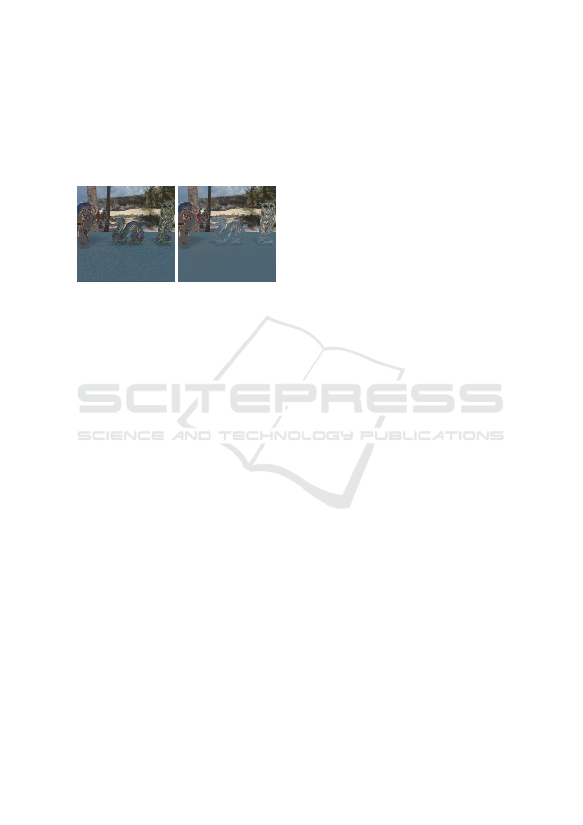
If an ideal refraction is encountered during the
propagation (fig. 3), we use the degradation strategy
(Evans and McCool, 1999). This strategy chooses
randomly one wavelength to continue the propagation
and stops the others. In this case, the throughput of
the chosen wavelength sample has to be scaled by the
number of wavelength samples carried by the path.
(a) 16 spp.
(b) 1,024 spp.
Figure 3: Refraction with degradation of paths which carry
64 wavelength samples at different spp (number of sample
per pixel).
3.6 Visualization
Since the spectral radiation of a scene at the input of
a sensor is refined in a spectral image, a color image
(RGB, false color, grayscale...) can be produced at
any moment for display purpose if needed. If we
change the sensor curve (XYZ, Camera RGB cur-
ves...) or the way to convert the spectral data to a
color, the simulation don’t have to be reseted. This
advantage can be useful for predictive rendering and
colorimetric validation. However, as stated in the
section 3.3, a good amount of channel is needed to
be accurate if the sensor response curve is not con-
stant on the spectral interval of the image. Another
interesting feature of this kind of rendering is to be
able to visualize in real time the output spectrum of a
pixel of the image (fig. 1).
4 THE STRAIGHTFORWARD
APPROACH OF THE PATH
TRACING ON GPU
Our GPU methods are based on the Streaming Path
Tracing (Antwerpen, 2011). The Multi Kernel im-
plementation is chosen because the performances are
more portable amongst the different GPU Vendors
(Davidovi
ˇ
c et al., 2014). Moreover, most of the in-
tersection libraries on GPU (Optix Prime (NVIDIA,
), Radeon-Rays (AMD, ) ...) do not provide an in-
tersection device function which would allow us to
integrate it in a Mega Kernel. So we need to split at
least some parts of the algorithm to communicate with
these libraries.
4.1 Algorithm
The straightforward approach would be to extend and
evaluate the path at each bounce. In this case, the
states of every wavelength sample of each path have
to be kept alive, since the full path is not known and
some values (spectral radiance and path throughput)
have to be accumulated.
To be efficient, a path has to be reused by at least
one wavelength sample per channel. When the num-
ber of channels will raise, this approach would lead us
to high memory consumption and latency problems,
since the states of each wavelength sample have to be
updated from the global memory at each bounce.
It should be noted that a Mega Kernel implemen-
tation does not solve these problems since the wave-
length sample states won’t be able to fit into the re-
gisters or the local memory. The only possibility is to
store them in the global memory.
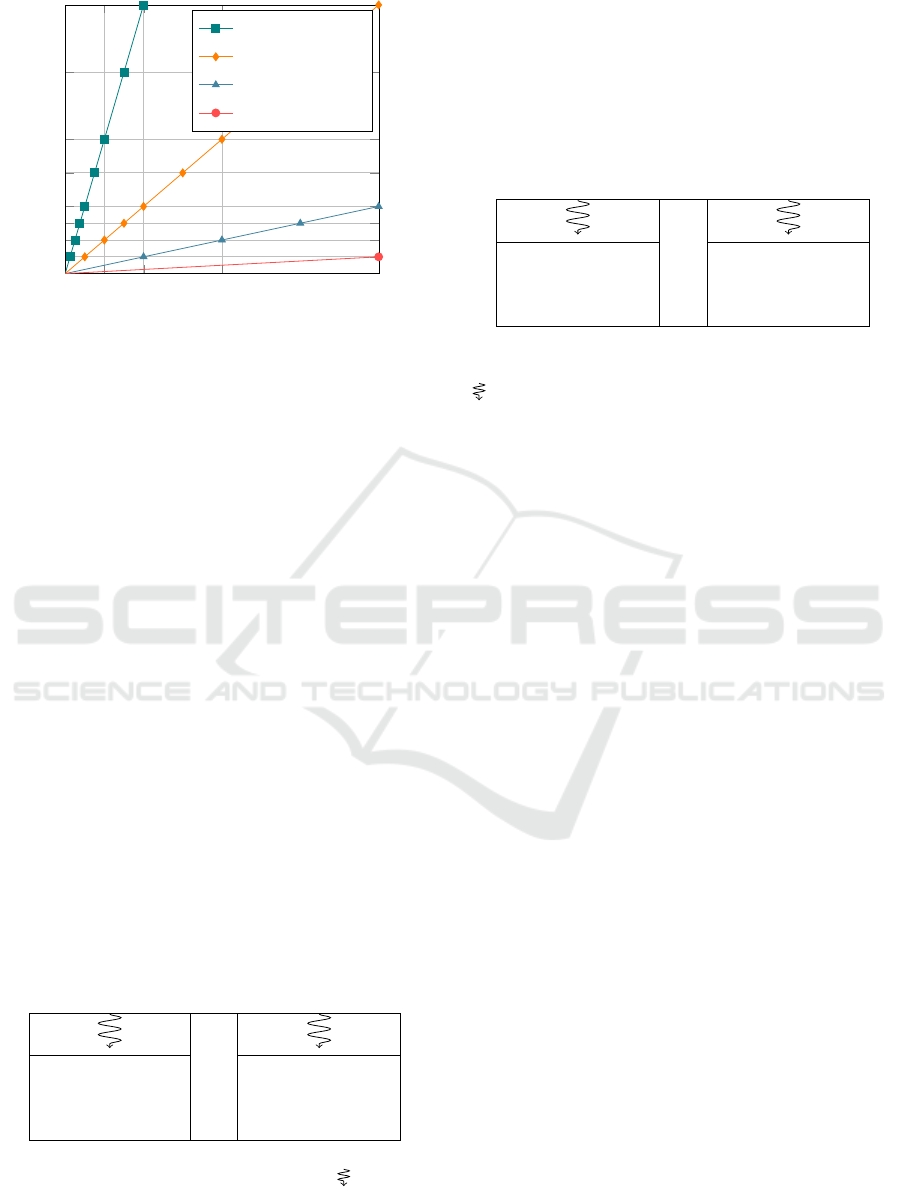
4.2 The Memory Consumption
The memory consumption of this method is proporti-
onal to the number of channels (fig. 4) since we need
to store for each thread:
• The path state which weights 32 bytes composed
by :
– The idle state.
– The current depth.
– The pixel index.
– The ray index.
– The random number generator.
– The spectral sample µ.
– The last material PDF (For MIS).
– The selected channel index in case of re-
fraction.
• For each channel, the wavelength sample state
which weights 16 bytes (4 padding bytes):
– The throughput.
– The spectral radiance.
– The direct light contribution (For a Multi Ker-
nel implementation, we need to add it later to
the spectral radiance if the shadow ray is not
occluded).
Interactive Hyper Spectral Image Rendering on GPU
75

256 512
1,024 2,048
2
4
6
8
12
16
24
32
Number of channels
Memory consumption in Gigabytes
2, 048
2
Threads
1, 024
2
Threads
512
2
Threads
256
2
Threads
Figure 4: Memory consumption of the Path Tracing for dif-
ferent threads pool sizes.
This is problematic because it limits the number of
channels and the size of the pool threads. We saw du-
ring our experiments that a size between 1, 024
2
and
2, 048
2
threads is required to reach the peak of perfor-
mance. A pool of 1, 024
2
threads would quickly limit
the number of channels (e.g. 512 channels for around
8.2 GB of memory footprint).
5 DPEPT: DEFERRED PATH
EVALUATION PATH TRACING
5.1 Algorithm
The DPEPT consists in two following steps:
1. The building and the saving of the full path.
2. The evaluation of the wavelength samples of the
saved paths.
To reduce the memory consumption, the wave-
length samples are evaluated per batch by reloading
their path (fig. 5). Since registers are scarce and pre-
cious resources (and they have to be spared for the
path evaluation), the state of a batch are stored in the
local memory to reduce latency (algorithm 1).
···
EvalPath(ω
0
, β
0
0
) EvalPath(ω
p
, β
p
0
)
.
.
.
.
.
.
EvalPath(ω
0
, β
0
b
) EvalPath(ω
p
, β
p
b
)
Figure 5: One path per work-item parallelization pattern
of a work-group for the paths evaluation. is a work
item (thread of the work group). EvalPath(ω
p
, β
p
b
) is the
evaluation of the path sample p for its wavelength sample
batch b (algorithm 1).
5.2 Parallelism over Wavelength
Samples Batches
Although the DPEPT was better than the straightfor-
ward method, the performance was not enough suf-
ficient. To improve the path evaluation step of the
DPEPT, a wavelength samples batches parallelization
pattern (fig. 6) has been developed.
···
EvalPath(ω
0
, β
0
0
) EvalPath(ω
0
, β
0
b
)
.
.
.
.
.
.
EvalPath(ω
p
, β
p
0
) EvalPath(ω
p
, β
p
b
)
Figure 6: Wavelength samples batches per work-item paral-
lelization pattern of a work-group for the paths evaluation.
is a work item (thread of the work group). EvalPath(ω
p
,
β
p
b
) is the evaluation of the path sample p for its wavelength
sample batch b (algorithm 1).
Instead of processing a path per work item (fig. 5),
the whole work group processes different wavelength
samples batch of the same path at the same time. This
way, the work group instruction coherence is nearly
perfect. And since the work items read exactly the
same path, the cache miss decreases and we can be-
nefit from the broadcast feature if it’s available.
However, in order to be fully utilized, the work-
group needs to have enough batch. On AMD har-
dware (16-wide SIMD units), when the number of
channels is less than 16, the version 1 (fig. 5) is better
than the version 2 (fig. 6).
5.3 The Memory Consumption
The memory consumption of this implementation is
dependent on the maximum number of bounces of a
path (fig. 7) since we need to store for each thread:
• The path state which weights 32 bytes composed
by :
– The idle state.
– The current depth.
– The pixel index.
– The ray index.
– The random number generator.
– The spectral sample µ.
– The last material PDF (for MIS).
– The selected channel index in case of re-
fraction.
GRAPP 2018 - International Conference on Computer Graphics Theory and Applications
76

• A number of vertex which each weights 80 bytes
(8 padding bytes) composed by:
– An integer to store some flags (if a shadow ray
was not occluded...).
– The material ID.
– The light ID.
– The direction to the light.
– The light sample PDF (The cosinus term and
the MIS weight are packed in the PDF).
– The outgoing direction to the light (BSDF
space).
– The ingoing direction (BSDF space).
– The outgoing direction (BSDF space).
– The surface self emission MIS weight.
– The material sample PDF (The cosinus term
and the MIS weight are packed in the PDF).
4 8
16
32 48
64
80
96
2
4
6
8
12
16
24
32
Number of Bounces
Memory consumption in Gigabytes
2, 048
2
Threads
1, 024
2
Threads
512
2
Threads
256
2
Threads
Figure 7: Memory consumption of the DPEPT implemen-
tation for different thread pool sizes.
GPUs don’t mostly support dynamic allocation on
the device side. And when they do, it’s strongly advi-
sed to not use this feature. Therefore for each thread,
a maximum of path vertex has to be preallocated on
the host side. Hopefully we do not need as much
bounce as channel. Therefore, regardless the number
of channels, a pool of 1, 024
2
threads with 32 boun-
ces will consume for around 2.6 GB. Although the
size of a path vertex will increase when complex ma-
terials (texture, volume...) will be added, there is still
plenty of room before reaching the level of memory
consumption of the straightforward approach.
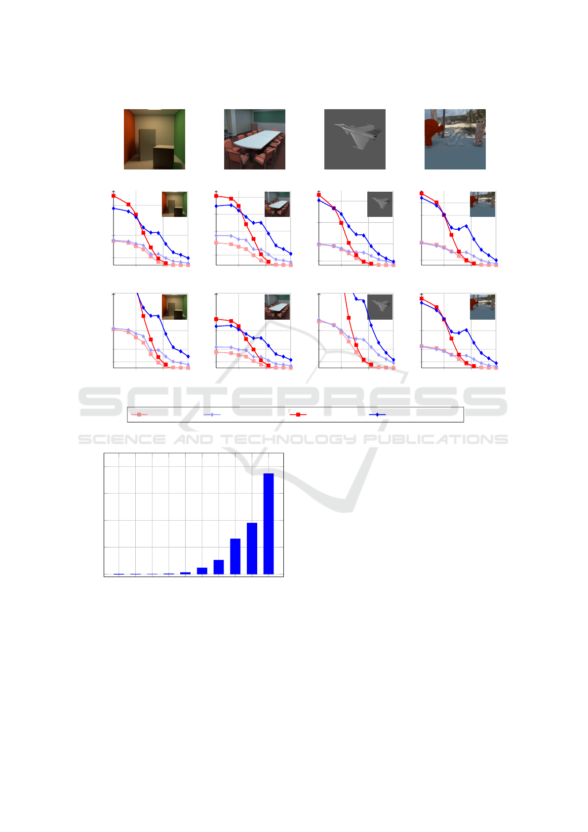
6 RESULTS
To compare the PT (conventional Path Tracing) and
the DPEPT methods, a benchmark (fig. 8) has been
made. It consists in measuring the number of paths
completed per second (raw performance) and the FPS
(interactivity) at different thread pool sizes and num-
ber of channels.
The benchmark (fig. 8) has been run on the follo-
wing scene:
• Cornell box: The maximum depth of this easy
indoor scene has been fixed at 5 bounces.
• Conference: The maximum depth of this medium-
complex indoor scene has been fixed at 8 bounces.
• Aircraft: An easy outdoor scene which is typically
used to dimension aircraft detection sensors. The
scene contains a spectral environment light gene-
rated by MATISSE (Simoneau et al., 2006). The
maximum depth has been fixed at 5 bounces.
• Statues: A medium-complex outdoor scene which
contains a refractive object and a spectral environ-
ment light converted from a rgb hdr image. The
maximum depth has been fixed at 16 bounces.
Except Suzanne (Blender) and the Aircraft (ON-
ERA), the other meshes come from (McGuire, 2017).
For a 1, 024
2
pool of thread with 16 bounces on
a Fury X (4GB of VRAM), a full HD image would
limit the number of channels to around 220 for the
DPEPT and to around 127 for the PT. Therefore, in
order to be not limited by the memory consumption
of the spectral image, the spatial image resolution was
fixed to 512x512.
When the number of channels is under 8, the per-
formance of our method is usually a bit subpar com-
pared to the Path Tracing. However, when the number
of channels raises, the Path Tracing is considerably
slower than our method.
Due to its lower memory consumption, the
DPEPT can render more channels than the straight-
forward Path Tracing approach which limits the size
of the thread pool.
For instance if we render a image with 512
spectral channels, the Path Tracing won’t be able to
allocate a thread pool size of 1, 024
2
on the Fury X
(4GB of VRAM). Our technique can easily reach the
size of 1, 024
2
threads and it is thus faster by around
38 times on average (fig. 9).
The results of the benchmark show us that our
method allows us to render at interactive frame rate
(around 10 FPS) a hyper spectral image (between 100
and 200 channels).
Interactive Hyper Spectral Image Rendering on GPU
77

Cornell Box.
Conference. Aircraft.
Statues.
8 100 1,000
5
20
40
.10
6
Samples . Second
−1
8 100 1,000
3
10
15
20
8 100 1,000
4
20
40
60
8 100 1,000
2
20
25
8 100 1,000
10
30
60
120
Number of Channels
FPS
8 100 1,000
10
30
60
120
8 100 1,000
10
30
60
120
8 100 1,000
10
30
60
120
PT (256
2
Threads) DPEPT (256
2
Threads) PT (1, 024
2
Threads) DPEPT (1, 024
2
Threads)
Figure 8: Benchmark with an AMD Fury X (VRAM: 4GB). The scaling of the x-axis is a logarithm base 2.
1 4
8
16 32 64
128 256 512
1024
0
20
40
60
80
−0.12
−6.63· 10
−2
2.26 · 10
−2
0.33
1.2
4.68
10.39
26.22
37.95
74.7
Number of channels
Speedup
Figure 9: Average DPEPT speedup of the raw performance
over the PT for the benchmark (fig. 8).
7 TECHNICAL DETAILS
We use SYCL to implement our rendering engine.
SYCL is the new royalty-free Khronos Group stan-
dard that allows to code in OpenCL in a single C++
source fashion. It lowers the burden of program-
mer by managing the data movement transaction bet-
ween the host and device. Therefore, the programmer
can focus on the optimization of his kernels. At the
moment there are three implementations of the stan-
dard: ComputeCpp (Codeplay, ), TriSYCL (Khronos-
Group, ) and SYCL-GTX (Žužek, ). We use the beta
of the Community edition of ComputeCpp, since it is
the most advanced implementation at the time of this
publication.
To compute the ray and shadow ray intersections,
we use Radeon-Rays. It is an AMD open source li-
brary for ray tracing. Like Optix Prime, we need
to provide a ray buffer, and the library returns a hit
point buffer. The library can use different back-ends:
Vulkan, OpenCL and Embree. We have chosen the
OpenCL back-end since we can use it via the intero-
perability feature of SYCL.
GRAPP 2018 - International Conference on Computer Graphics Theory and Applications
78

8 CONCLUSION
In this article, we endeavour to simulate efficiently
and accurately spectral image (fig. 1). The previ-
ous works in spectral rendering don’t fulfill the requi-
rements (section 3.1). Therefore, a new framework
(section 3) has been described to render a spectral
image composed with K number of channels.
The rendering of a such spectral image will lead
us to three major issues: the computation time, the
footprint of the spectral image, and the memory con-
sumption of the algorithm. The computation time can
be drastically reduced by the use of GPUs, however,
their memory capacity and bandwidth (compared to
their compute power) are limited. When the num-
ber of channels will raise, the straightforward method
(section 4) will lead us to high memory consumption
and latency problems.
To overcome these problems, we propose the
DPEPT (section 5.1) which consists in decoupling the
path evaluation from the path generation. The me-
mory consumption of this approach is not dependent
on the number of channels. Its path evaluation step
can be efficiently parallelized (section 5.2). Our met-
hod outperforms the straightforward approach when
the spectral resolution of the simulated image raises.
Our contributions enable to render multi, hyper and
even ultra (more than 1,000 channels) spectral image.
Interactive frame rate of hyper spectral image rende-
ring can be achieved for easy and medium complex
scene.
However we think there are still room to improve
the compute time and the convergence of the simula-
tion. More over, the footprint of the spectral image
problem is not yet solved, therefore it can limit the si-
mulation if the spectral image is too big to fit in the
global memory of a GPU.
9 FUTURE WORK
The possible future work would consist in:
• Improving the compute time. We have made the
assumption that it’s needed to compute one wa-
velength sample per channels per path, maybe we
can find a better tradeoff between the number of
wavelength samples to evaluate per path and the
number of path to trace.
• Investigating the feasibility of the spectral MIS
(Wilkie et al., 2014) for paths which carry a large
number of wavelength samples on GPU. It would
improve the convergence of the algorithm when
using high wavelength dependent materials.
• Exploring the viability of Out-of-Core methods to
refine the spectral image.
• Working on an efficient and compact data struc-
ture to refine the spectral output. Right now, the
output are stored in a spectral image composed
with K number of channel (3d image) which is
computational-wise and memory-wise inefficient.
• Studying an efficient multi GPU parallelization
pattern for a spectral image rendering.
ACKNOWLEDGEMENTS
This work has been funded by the Provence-Alpes-
Côte d’Azur (PACA) French region and ONERA.
REFERENCES
AMD. Radeon-rays. https://github.com/GPUOpen-
Libraries AndSDKs/RadeonRays_SDK.
Antwerpen, D. V. (2011). Improving SIMD Efficiency for
Parallel Monte Carlo Light Transport on the GPU.
Hpg 2011, (X):10.
Codeplay. Computecpp. https://www.codeplay.com/ pro-
ducts/computesuite/computecpp.
Coiro, E. (2012). Global Illumination Technique for Air-
craft Infrared Signature Calculations. Journal of Air-
craft, 50(1):103–113.
Davidovi
ˇ
c, T., K
ˇ
rivánek, J., Hašan, M., and Slusallek, P.
(2014). Progressive Light Transport Simulation on the
GPU. ACM Transactions on Graphics, 33(3):1–19.
Evans, G. F. and McCool, M. D. (1999). Stratified wave-
length clusters for efficient spectral Monte Carlo ren-
dering. In Proceedings of the 1999 conference on
Graphics interface ’99, pages 42–49.
Kajiya, J. T. (1986). The Rendering Equation. SIGGRAPH
Comput. Graph., 20(4):143–150.
KhronosGroup. Trisycl. https://github.com/triSYCL/ tri-
SYCL.
Laine, S., Karras, T., and Aila, T. (2013). Megakernels Con-
sidered Harmful: Wavefront Path Tracing on GPUs.
mediatech.aalto.fi, (typically 32).
McGuire, M. (2017). Computer graphics archive.
https://casual-effects.com/data.
Novák, J., Havran, V., and Dachsbacher, C. (2010). Path
Regeneration for Interactive Path Tracing. Euro-
graphics 2010, pages 1–4.
NVIDIA. Optix prime. https://developer.nvidia.com/optix.
Purcell, T. J., Buck, I., Mark, W. R., and Hanrahan, P.
(2002). Ray tracing on programmable graphics har-
dware. ACM Transactions on Graphics (TOG) - Pro-
ceedings of ACM SIGGRAPH 2002, 21:703–712.
Radziszewski, M., Boryczko, K., and Alda, W. (2009). An
improved technique for full spectral rendering. Jour-
nal of WSCG, 17(1-3):9–16.
Interactive Hyper Spectral Image Rendering on GPU
79

Rohde, R. A. (2007). Atmospheric transmission.
https://en.wikipedia.org/wiki/File:Atmospheric_
Transmission.png.
Simoneau, P., Caillault, K., Fauqueux, S., Huet, T., Kra-
pez, J.-C., Labarre, L., Malherbe, C., and Miesch, C.
(2006). Matisse: Version 1.4 and future developments.
6364.
Žužek, P. Sycl-gtx. https://github.com/ProGTX/sycl-gtx.
Veach, E. and Guibas, L. J. (1995). Optimally combining
sampling techniques for Monte Carlo rendering. Pro-
ceedings of the 22nd annual conference on Computer
graphics and interactive techniques - SIGGRAPH ’95,
pages 419–428.
Whitted, T. (1979). An improved illumination model
for shaded display. ACM SIGGRAPH Computer
Graphics, 13(2):14.
Wilkie, A., Nawaz, S., Droske, M., Weidlich, A., and Ha-
nika, J. (2014). Hero Wavelength Spectral Sampling.
Computer Graphics Forum, 33(4):123–131.
APPENDIX
Algorithm 1: Evaluation of the path ω for the wa-
velength batch β.
Local Memory:
L : Spectral radiances of the batch β.
τ : Path throughputs of the batch β.
Global Memory:
V : Saved Paths vertices.
I : Spectral Image.
Function:
At the vertex v for the wavelength λ:
Env(v, λ) : Environment light contribution.
NEE(v, λ) : Direct light contribution.
Le(v, λ) : Self emission of the surface.
T (v, λ) : Path throughput.
Function EvalPath(ω, β):
// Initialize the batch
foreach λ ∈ β do
L[λ] = 0
τ[λ] = 1
end
// Evaluation of the batch
foreach v ∈ V [ω] do
if v is a miss vertex then
// Environment light
foreach λ ∈ β do
L[λ] += τ[λ] * Env(v, λ)
end
else
foreach λ ∈ β do
// Next event estimation
L[λ] += τ[λ] * NEE(v, λ)
// Surface self emission
L[λ] += τ[λ] * Le(v, λ)
// Update the throughput
τ[λ] *= T (v, λ)
end
end
end
// Refine the spectral image
foreach λ ∈ β do
Refine(I[ω. pixelID], L[λ])
end
return
GRAPP 2018 - International Conference on Computer Graphics Theory and Applications
80