
Lowest Unique Bid Auctions with Resubmission Opportunities
Yida Xu and Hamidou Tembine
Learning & Game Theory Laboratory, New York University Abu Dhabi, United Arab Emirates
Tandon School of Engineering, New York University, U.S.A.
Keywords:
LUBA, Auction, Game Theory, Imitative Learning, Reinforcement Learning.
Abstract:
The recent online platforms propose multiple items for bidding. The state of the art, however, is limited
to the analysis of one item auction. In this paper we study multi-item lowest unique bid auctions (LUBA)
in discrete bid spaces under budget constraints. We show the existence of mixed Bayes-Nash equilibria for
an arbitrary number of bidders and items. The equilibrium is explicitly computed in two bidder setup with
resubmission possibilities. In the general setting we propose a distributed strategic learning algorithm to
approximate equilibria. Computer simulations indicate that the error quickly decays in few number of steps
by means of speedup techniques. When the number of bidders per item follows a Poisson distribution, it is
shown that the seller can get a non-negligible revenue on several items, and hence making a partial revelation
of the true value of the items.
1 INTRODUCTION
With the increasing impact of information technology,
the traditional structure of economic and financial
markets has been revolutionized. Today, the market
includes millions of economic agents worldwide and
reaches an annual transaction of billions U.S. dollars.
In this paper, we study a little-studied type auction
which is called lowest unique bid auction (LUBA).
Because of a limited number of items provided by the
auctioneers and budget restrictions, bidders need to
manage their behaviors in a strategic way.
Literature Review
Auctions: In 1961 in the work of Vickrey (Vick-
rey, 1961), the theory of auctions as games of in-
complete information is first proposed. Auctions
with homogeneous valuation distributions (symmet-
ric auctions) and self-interested non-spiteful bidders
are well-investigated in the literature. However, auc-
tions with asymmetric bidders remain a challenging
open problem (see (Maskin and Riley, 2000; Lebrun,
1999; Lebrun, 2006) and the references therein). In
asymmetric auction scenarios, the expected “revenue
equivalence theorem” ( Myerson 1981) does not hold,
i.e., the revenue of the auctioneer depends on the
auction mechanism employed. In addition, there is
no ranking revenue between the auction mechanisms
(first, second, English or Deutch). Most of research
articles (Bang-Qing, 2003; C. Yi, 2015 ; N. Wang,
2014; Rituraj and Jagannatham, 2013) on multi-item
auctions works provide computer simulation or nu-
merical experiments results. However, no analysis
of the outcome of the multi-item auction is available.
There is no analysis of the equilibrium seeking algo-
rithm therein.
LUBA: LUBA is different from the lowest cost auc-
tion called procurement auction which is widely used
in e-commerce(J. Zhao, 2015), hybrid cloud comput-
ing or in demand-supply matching in power grids (R.
Zhou, 2015). As a special case of unmatched bid auc-
tions, the single-item LUBAs have been studied by
other researchers (H. Houba, 2011; Stefan and Nor-
man, 2006; Rapoport, 2007; Erik, 2015; J.Eichberger,
2008).
The authors (Stefan and Norman, 2006) run lab-
oratory experiments with one bid min bid auctions.
They consider the results of a Monte Carlo simula-
tion under the restriction of one bid per player. The
work in (Erik, 2015) considers a lowest unique posi-
tive integer experiment in a single bid per player set-
ting. The observed behaviors are compared with the
solution of a Poisson game. The authors in (Rapoport,
2007) consider both high and low unique bid auctions,
and they also assume that bidders are restricted to a
single bid. A numerical approximation of the solu-
tion for a game-theoretic model is provided. The so-
330
Xu, Y. and Tembine, H.
Lowest Unique Bid Auctions with Resubmission Opportunities.
DOI: 10.5220/0006548203300337
In Proceedings of the 10th International Conference on Agents and Artificial Intelligence (ICAART 2018) - Volume 2, pages 330-337
ISBN: 978-989-758-275-2
Copyright © 2018 by SCITEPRESS – Science and Technology Publications, Lda. All rights reserved

lutions are compared with the results of a laboratory
experiment. (J.Eichberger, 2008; J.Eichberger, 2015;
J. Eichberger, 2016) conduct field experiments on
Lowest-Unmatched Price Auctions with high prizes
involving large numbers of participants (tens and hun-
dreds of thousands). The work in (Dong-Her, 2011)
discusses security and privacy issues of multi-item re-
verse Vickrey auction. They provide more secure pro-
tocol design. Most of the above works restrict the
number of submissions per bidder to one. The re-
cent focus within the auction field has been multi-item
auctions. The bidder can also place multiple bids for
each item. It has been of practical importance in In-
ternet auction sites and has been widely executed by
them.
2 PROBLEM STATEMENT
A LUBA operates under the following three main
rules: Whoever bids the lowest unique positive bid
wins; If no unique bid exits then no one wins; No
participant can see bids placed by other participants.
“Lowest unique bid” means the lowest amount that
nobody else has bid.
In the multi-item LUBA, there are n ≥ 2 bidders
exerting effort for m items (objects) proposed by the
auctioneers. Each bidder has the information as fol-
low. Valuation vector: Each bidder j has a vector of
values v
j
= (v
ji
)
i∈I
, for assessing the worth of each
object i offered for the auction. The random variable
v
ji
has support [v, ¯v] where 0 < v < ¯v. A bidder may
have his/her own valuation vector but not the valua-
tion vector of the others. Budget: Each bidder j has a
initial total budget of
¯
b
j
to be used for all items. Reg-
istration fee: To participate in the LUBA, each bidder
needs to pay a one time registration fee c
r
. Submis-
sion fee: To participate in the auction on item i, he/she
needs to pay a submission fee c
i
for each submission.
Note that each bidder can resubmit bids a certain
number of times subject to his or her available bu-
ject. If bidder j has (re)submitted n
ji
times on item i,
his/her total submmission/bidding cost would be n
ji
c
i
in addition to the registration fee. The set that con-
tains all the bids of bidder j on item i is denoted by
B
ji
⊂ N. Thus, we can obtain the set of bidders who
are submitting b on item i by N
i,b
= { j ∈ J | b ∈ B
ji
}.
We use |N
i,b
| to represent the cardinality of N
i,b
. Ob-
viously, |N
i,b
| = 1 yields that b was chosen by only
one bidder. Then, the set of all positive natural num-
bers that were unique on item i can be calculated by
B
∗
i
= {b > 0 | |N
i,b
| = 1}. B
∗
i
=
/
0 yields no winner
on item i at that round. If B
∗
i
6=
/
0, there is a winner
on item i, and the winning bid is inf B
∗
i
. At the same
time, the winner can be calulated by j
∗
∈ N
i,infB
∗
i
.
2.1 The Payoff of Participants
The cost of bidder j on item i consists of the registra-
tion fee c
r
, the submission fee |B
ji
|∗c
i
, and the bid fee
which is conditional on moves by the other bidders. If
he/she is the winner, the bid fee is infB
∗
i
calculated by
the proceeding subsection. Losing the LUBA yields
no bid fee. Thus, the payoff of bidder j on item i at
a round would be r
ji
= v
ji
− |B
ji
|c
i
− inf B
∗
i
− c
r
, if j
is a winner on item i, and r
ji
= −|B
ji
|c
i
− c
r
, if j is
not a winner on item i. The payoff of bidder j on item
i is zero if B
ji
is reduced to {0} (or equivalently the
empty set). Thus, it is easy to conclude that
r
ji
(B)
= [−c
r
− c
i
|B
ji
| −(v
ji
− b
ji
)1l
{b
ji
=infB
∗
i
}
]1l
{B
ji
6={0}}
,
(1)
where the infininum of the empty set is zero. Over-
all, the total payoff of bidder j is r
j
(B) =
∑
i∈I
r
ji
(B).
The instant payoff of the auctioneer of item i can be
calculated by
r
a,i
=
∑
j
c
r
1l
{B
ji
6=
/
0}
+ infB
∗
i
+
∑
j=1
|B
ji
|c
i
!
− v
a,i
,
where v
a,i
is the realized valuation of the auctioneer
for item i. Obviously, the instant payoff of the auc-
tioneer of a set of item I is r
a,I
=
∑
i∈I
r
a,i
. In terms of
reward seeking, bidders are interested in optimizing
their payoffs, and auctioneers are interested in their
revenue.
3 SOLUTION APPROACH
Since the game is of incomplete information, the
strategies of participating in the game must be spec-
ified as a function of the information structure. We
introduce the definition of pure strategy and mixed
strategy as follows.
Definition 1. A pure strategy of a bidder is a choice
of a subset of natural numbers contingent on the own-
value and own-budget. Thus, given a bidder’s own
valuation vector v
j
= (v
ji
)
i
, the bidder j will choose
an action (B
ji
)
i
that satisfies the budget constraints,
which is
∑
i
c
r
1l
{B
ji
6={0}}
+
m
∑
i=1
[infB
∗
i
]1l
B
ji
∩[infB
∗
i
]
+
m
∑
i=1
|B
ji
|c
i
≤
¯
b
j
.
The set of multi-item bid space for bidder j is
B
j
(v
j
,
¯
b
j
) = {(B
ji
)
i
| B
ji
⊂ {0, 1, . . . ,
¯
b
j
− c
r
},
∑
i
c
r
1l
{B
ji
6={0}}
+
∑
m
i=1
[infB
∗
i
]1l
B
ji
∩[infB
∗
i
]
+
∑
m
i=1
|B
ji
|c
i
≤
¯
b
j
}.
Lowest Unique Bid Auctions with Resubmission Opportunities
331

• A pure strategy is a mapping v
j
7→ B
j
⊂ N. A con-
strained pure strategy is a mapping v
j
7→ B
j
∈ B
j
.
• A mixed strategy is a probability measure over the
set of pure strategies.
The action set B
j
(v
j
,
¯
b
j
) is finite because of bud-
get limitations; hence, a bid b
ji
∈ B
ji
is less than
min(
¯
b
j
, v
ji
− c
r
). We define a solution concept of
the above game with incomplete information: Bayes-
Nash equilibrium.
Definition 2. A mixed Bayes-Nash strategy equilib-
rium is a profile (s
j
(v
j
))
j
such that for all bidders j
E
s
j
,s
− j
r
j
(B
j
(v
j
), B
− j
| v
j
) ≥ E
s
0
j
,s
− j
r
j
(B
0
j
, B
− j
| v
j
), for
any strategy s
0
j
.
The information structure of the auction is as fol-
lows. Each bidder knows its own-value and own-bid
but not the valuation of the other bidders. Each bidder
has the valuation cumulative distribution of the others.
The structure of the game is common knowledge. We
are interested in the equilibria, the equilibrium pay-
offs of the bidders, and the revenue of the seller.
Existence of Bayes-Nash Equilibrium
Proposition 1. The multi-item Bayesian LUBA game
(without resubmission) but with arbitrary number of
bidders has at least one Bayes-Nash equilibrium in
mixed strategies under budget restrictions.
Proposition 1 provides the existence of at least one
Bayes-Nash equilibrium. However, it does not tell us
what are those equilibria or how can we target them.
The next subsection computes some of the equilibria
in specific setups.
Computation of Bayes-Nash Equilibrium
Proposition 2. Any strategy b
j
such that b
ji
>
min
v
ji
− ˜c − 1,
¯
b
j
is strictly dominated by strat-
egy“0”. If v
ji
< c, bidder j is better off of not par-
ticipating on item i.
Thus, the bid space of j can be reduced to
∏
m
i=1
{0, 1, 2, . . . , min(v
ji
− ˜c − 1,
¯
b
j
)}. Now, we ana-
lyze some of the equilibria in specific setups.
Two Participants. Let n = 2, and the action space is
restricted to {0, 1, 2, . . . , v − ˜c}, where ˜c = c + c
r
.
Proposition 3. Suppose v > ˜c + 1 and n = 2. With
the non-participation option, i.e., when the bid can
be zero, (0, . . . , 0, 1, 0, . . . , 0) and its permutations are
equilibria.
We can easily derive proposition 3 from the payoff
matrix, which is shown in Table 1.
Table 1: Payoff matrix of 2 bidders bidding 1 item.
0 1 2 3
0 0, 0 (0, v − ˜c − 1)
∗
0, v − ˜c − 2 0, v − ˜c − 3
1 (v − ˜c − 1, 0)
∗
− ˜c,−˜c v − ˜c − 1,− ˜c v − ˜c − 1,− ˜c
2 v − ˜c − 2,0 − ˜c,v− ˜c − 1 − ˜c, −˜c v − ˜c − 2,− ˜c
Proposition 4. When the budgets are identical and
equal to k, and n = 2, There is a partially mixed equi-
librium which is symmetric and is explicitly given by
(X
0
, X
1
, X
2
, . . . , X
k
) = (
˜c
v − 1
, 1 −
˜c
v − 1
, 0, . . . , 0).
Three Participants. With three participants, the ac-
tion profile (1, 1, 1) is not an equilibrium anymore: if
players 1 and 2 bid 1 cent then player’s 3 best re-
sponse is to bid 2 and player 3 will be the winner
of the auction. The game is not a dominant solvable
game.
Table 2: Payoff matrix of 3 bidders targetting 1 item.
0 1
0 0, 0, 0 (0, v − ˜c − 1, 0)
∗
1 (v − ˜c − 1, 0, 0)
∗
− ˜c,− ˜c,0
0 1
0 (0, 0, v − ˜c − 1)
∗
0, − ˜c, −˜c
1 − ˜c,0, −˜c − ˜c,− ˜c, − ˜c
Proposition 5. When the budgets are identical and
n ≥ 3, There is a partially mixed equilibrium which is
symmetric and is explicitly given by
(X
0
, X
1
, X
2
, . . . , X
k
) = (
n−1
r
˜c
v − 1
, 1 −
n−1
r
˜c
v − 1
, 0, . . . , 0).
3.1 Multi-item LUBA Game
Now we investigate the property of multi-item LUBA
game. First, we analyze a simple setup, then we ex-
tend it to a general form. We assume n = 2, b
1
= 4+ ˜c,
and b
2
= 3 + ˜c. Thus, the action profiles of each bid-
der can be expressed as A
1
= {b
1
: b
11
+b
12
≤ 4} and
A
2
= {b
2
: b
21
+ b
22
≤ 3}. More specifically,
A
1
= {(0, 0), (1, 0), (0, 1), (2, 0), (1, 1), (0, 2), (3, 0),
(0, 3), (2, 1), (1, 2), (4, 0), (3, 1), (0, 4), (1, 3), (2, 2)}
A
2
= {(0, 0), (1, 0), (0, 1), (2, 0), (0, 2), (1, 1), (3, 0),
(0, 3), (1, 2), (2, 1)}
From the action files, we can derive that
{(0, 0), (1, 1)}, {(1, 1), (0, 0)}, {(0, 1), (1, 0)},
and {(1, 0), (1, 0)} are pure Nash equilibria.
For the extended version, the game can be de-
fined as G(J, (b
j
)
j∈J
, (c, c
r
), m, (F
j
)
j∈J
). When
b
j
is given, we can derive that the action
profile A
j
= D
0
∪ D
1
∪ D
2
∪ . . . ∪ D
b
j
, where
D
k
= {(a
1
, . . . , a
m
) ∈ N
m
| a
i
≥ 0,
∑
m
i=1
a
i
= k} is the
set of all possible decomposition of the integer k.
ICAART 2018 - 10th International Conference on Agents and Artificial Intelligence
332

Proposition 6. If b
j
> 1 + ˜c, the set of pure
Nash equilibria of multi-item auction game
G(J, (b
j
)
j∈J
, (c, c
r
), m, (F
j
)
j∈J
), n ≥ 1, m ≥ 1
without resubmission is the set of matrices
b
11
b
12
b
13
. . . b
1m
b
21
b
22
b
23
. . . b
2m
b
31
b
32
b
33
. . . b
3m
. . . . . . . . . . . . . . . . . . . . . . . .
b
n1
b
n2
b
n3
. . . b
nm
such that ∀i, j, b
ji
∈ {0, 1}, ∀i ∈ {1, . . . , m},
∑
n
j=1
b
ji
=
1 and ∀ j ∈ {1, . . . , n},
∑
m
i=1
b
ji
≤
b
j
− ˜c. The pure
Nash equilibria are also global optima of the game.
3.2 Learning Algorithm
Imitative learning plays a role in many applications
(Tembine, 2012) such as security & reliability, cloud
networking, power grid and evolution of protocols
and technologies. It has been successfully utilized in
order to capture human learning and animal behav-
ior. We calculate the instant payoff of bidder j tar-
geting item i at tth round through R
t
ji
= −c
r
− c +
1l
j wins
(v
ji
− b
t
ji
). Bidder j wins item i at round t if
the placing bid b
t
ji
is the lowest unique bid on item i.
R
t
ji
= 0 if bidder j does not participate to item i. This
algorithm below describes how to update the reward
and the strategy in the bid space.
ˆ
R
t
ji
(k) is the estima-
tion of the reward a bidder j can obtain by holding the
bid k. Denote the estimate of R
t
ji
(k) by
ˆ
R
t
ji
(k) .
Algorithm 1: The Imitative learning algorithm.
Initialization: Generate
ˆ
R
0
ji
(0),
ˆ
R
0
ji
(1), . . . ,
ˆ
R
0
ji
(
¯
b(0)) from the uniform distribution.
For Round t +1:
1.Update the reward estimation:
ˆ
R
t
ji
(k) :
ˆ
R
t+1
ji
(k) =
ˆ
R
t
ji
(k) +1l
{b
t
ji
=k}
α
t
ji
(R
t
ji
−
ˆ
R
t
ji
(k))
2.Update the mixed strategy: X
t+1
ji
(k) = X
t
ji
(k)(1 + λ
t
ji
)
ˆ
R
t
ji
(k)
3.Normalize the mixed strategy.
Iterate until convergence.
The next result provides a convergence of the al-
gorithm to pure equilibria.
Proposition 7. If the algorithm starts from interior
point, it converges to an ending point in a stable
steady state of the replicator equation. This counts
for an arbitrary number of participants. Therefore it
is a Nash equilibrium. In the asymmetric case, the
mixed equilibrium is unstable and the algorithm con-
verges to one of pure Nash equilibria.
We give a simple example to show that the mixed
equilibrium is unstable, and the algorithm converges
to one of pure Nash equilibria. We analyze the situa-
tion where n = 2, v = 4, c = 1. In this specific parame-
ter setting, the ordinary differential equations (ODEs)
𝑋
1𝑖
(1)
𝑋
2𝑖
(1)
Figure 1: The vector field of ODEs where n = 2, v = 4,
c = 1.
are given by
˙
X
1i
(1) = X
1i
(1)(1 − X
1i
(1))(2 − 3X
2i
(1))
˙
X
2i
(1) = X
2i
(1)(1 − X
2i
(1))(2 − 3X
1i
(1))
Figure 1 shows the vector field of the ODEs. By an-
alyzing the vector field, we can observe that the algo-
rithm always converges to one of pure Nash equilibria
except the symetric situation; however, the probabil-
ity of symmetric situation is zero.
Proposition 8. In the symmetric case, the mixed equi-
librium is stable and the dynamical system converges
to it. However, the probability of obtaining equal
numbers by stochastic processes is nearly zero.
4 EXPERIMENT
In this part, we do experiments to show the effective-
ness of the imitative learning algorithm. First, we
present a numerical investigation focusing on learn-
ing symmetric equilibria for two bidders setting; then,
we extend to the asymmetric situation. Table 3 shows
the experiment setting. We compare and contrast the
results with the theory value presented in proposition
4.
Table 3: Summary of two bidders setting.
Symbol Setting
n 2
I 1
c 1
b
min
1
Initial of
ˆ
R
0
ji
[1 1 1]
Budget Static budget constraint
As shown in Figure 2, the proposed algorithm can
effectively learn the Nash equilibrium at a fast conver-
gence rate. More specifically, for big v, the learning
algorithm converges in a few steps. For the asymmet-
ric situation, the experiments in Figure 3 show that
the learning process can also converge to one of pure
equilibria in a few steps.
Lowest Unique Bid Auctions with Resubmission Opportunities
333
Bid
Cumulative distribution function
𝑣 = 4
𝑣 = 10
𝑣 = 200
𝑣 = 1000
1𝑠𝑡 𝐼𝑡𝑒𝑟𝑎𝑡𝑖𝑜𝑛 1000𝑡ℎ 𝐼𝑡𝑒𝑟𝑎𝑡𝑖𝑜𝑛
10𝑡ℎ 𝐼𝑡𝑒𝑟𝑎𝑡𝑖𝑜𝑛
8000𝑡ℎ 𝐼𝑡𝑒𝑟𝑎𝑡𝑖𝑜𝑛
(𝑛 = 2)
Figure 2: Nash equilibrium. The red squares present the
strategy learned by the proposed algorithm and the green
stars represent the theoretical equilibrium.
10𝑡ℎ 𝐼𝑡𝑒𝑟𝑎𝑡𝑖𝑜𝑛
80𝑡ℎ 𝐼𝑡𝑒𝑟𝑎𝑡𝑖𝑜𝑛
Probability mass function
𝑣 = 4
𝑣 = 10
𝑣 = 200
𝑣 = 1000
Bid
𝑛 = 2
Figure 3: Learned strategies. The red squares present bidder
1’s learned strategy under the proposed algorithm and the
green stars represent bidder 2’s learned strategy.
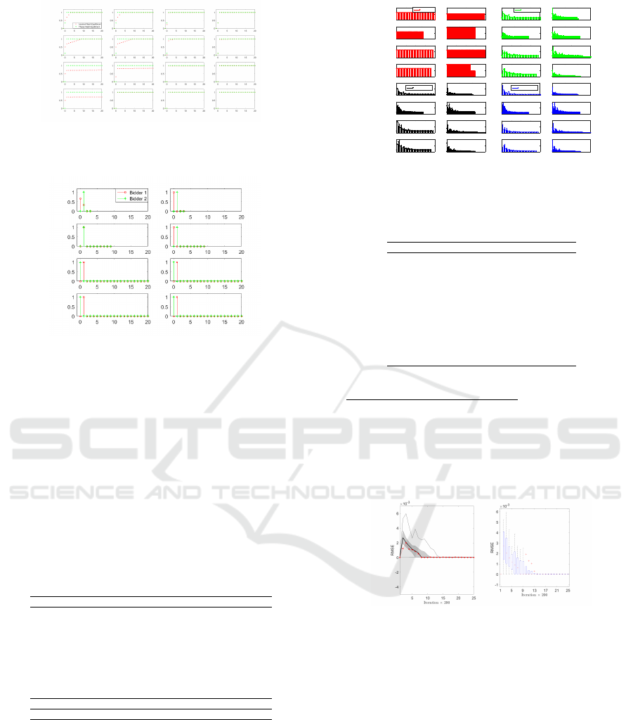
For multi-item under budget constrains, we also
do a simulation experiment to show the performance
of the proposed learning algorithm. The experiment
settings are shown in Table 4. We utilize a dynamic
setting with changing budget in this experiment by
setting different v
ji
and different initial budget. Con-
sidering the resources of item is limited, we also as-
sign resources of each item. Figure 4 shows the re-
sults.
Table 4: Summary of Multi-Items Experiment Setting.
Symbol Setting
N 4
I 2
c 1
b
min
1
Resource for item 1 and 2 [2000 1500]
Initial of Budget [100 120 80 90]
Initial of
ˆ
R
0
ji
0.0001
v for j ∈ {1, 2, 3, 4} [40,102],[42,109],[38,100],[36,110]
¯
b
ji
min(v
ji
, budget
ji
)
Assumption Description
Budget Budget evolves with the iteration.
4.1 Statistic Properties
In order to show the robustness of the proposed algo-
rithm, we do an experiment analysis under the static
budget constraint and analyze its statistic properties.
Table 5 presents the experiment setting.
We evaluate the convergence rate by introduc-
ing the root-mean-square error (RMSE). The prob-
ability distributions of sequential round strategies
0
10 20
30
40
0
0.1
0.2
Iteration 1800
0
50
100 150
0
0.05
0.1
0
20
40
60
0
0.05
0.1
0
50
100 150
0
0.02
0.04
0
10 20
30
40
0
0.05
0.1
0
50
100
0
0.05
0.1
0
10 20
30
40
0
0.05
0.1
0
50
100 150
0
0.05
0.1
0
10 20
30
40
0
0.1
0.2
Iteration 2000
0
50
100 150
0
0.05
0.1
0
20
40
60
0
0.05
0.1
0
50
100 150
0
0.02
0.04
0
10 20
30
40
0
0.1
0.2
0
50
100
0
0.05
0.1
0
10 20
30
40
0
0.1
0.2
0
50
100 150
0
0.05
0.1
Item1
Item2
Item1 Item2
0
10 20
30
40
0
0.02
0.04
Iteration 1
0
50
100
0
0.01
0.02
0
20
40
60
0
0.02
0.04
0
50
100 150
0
0.005
0.01
0
10 20
30
40
0
0.02
0.04
0
20
40
60 80
0
0.01
0.02
0
10 20
30
40
0
0.02
0.04
0
50
100 150
0
0.005
0.01
0
10 20
30
40
0
0.05
0.1
Iteration 1500
0
50
100 150
0
0.02
0.04
0
20
40
60
0
0.05
0.1
0
50
100 150
0
0.02
0.04
0
10 20
30
40
0
0.05
0.1
0
50
100
0
0.05
0
10 20
30
40
0
0.05
0.1
0
50
100 150
0
0.05
0.1
Bidder1
Bidder2
Bidder2
Bidder3
Bidder1
Bidder4
Bidder3
Bidder4
Probability mass function
Bid
Figure 4: Probability mass function of four players and two
items in the auction system with budget update.
Table 5: Summary of Experiment Setting.
Symbol Setting
N 4
I 1
α 0.1
λ 0.1
c 1
b
min
1
Initial of X
0
ji
Uniform distribution
Initial of
ˆ
R
0
ji
Unidrnd(20,1,Budget)
v
ji
for j ∈ {1, 2, 3, 4} [147,165,170,177]
¯
b
j
i for j ∈ {1, 2, 3, 4} [100,100,100,100]
Budget Static Budget Constraint
are utilized to calculate the RMSE. RMSE
t,t−1
=
q
∑
N
j=1
∑
¯
b
j
(t)
k=1
(X
t
ji
(k) − X
t−1
ji
(k))
2
. In order to analyze
the statistic property of the experiment results, we re-
conduct the experiment 200 times using the experi-
ment setting in the Table 5. The analysis of the statis-
tic properties are shown in Figure 5.
Figure 5: Statistic information on the RSME of the strate-
gies.
Figure 5 presents the distribution of RMSE (per-
centiles P5 P25 P50 P75 P90) obtained from the pro-
posed learning algorithm. The results in this figure
show all the repeat experiment converge to zero and a
narrow distribution of RMSE over the whole period.
4.2 Impact of Parameters
We investigated the impact of the parameters in the
proposed learning algorithm described in Sect.3.2.
Table 6 shows experiment setting details. Figure 6
and 7 present the statistic properties of RMSE evo-
lution obtained by the proposed learning algorithm.
Compared to α = 0.1 and λ = 0.1, the results show
ICAART 2018 - 10th International Conference on Agents and Artificial Intelligence
334

a fast convergence rate. The Boxplot shows that the
large parameter setting results less outliers in the ex-
periment results. According to the results in Figure
6 and 7, the parameter α and λ influence the conver-
gence of the proposed algorithm equally and a large α
can reduce disturbance and outliers more effectively.
Table 6: Summary of Experiment Setting in Parameters Im-
pact Investigation.
Symbol Original Setting Compared Setting
α 0.1 1
λ 0.1 1
Others Same as Table 5
Figure 6: Statistic information on RSME on strategies.
Figure 7: Statistic information on RSME.
5 LUBA WITH RESUBMISSION
In this section, we assume that each bidder can resub-
mit bids a certain number of times subject to her avail-
able budget, each resubmission for item i will cost c
i
.
If bidder j has (re)submitted n
ji
times on item i, his
or her total submission cost would be n
ji
c
i
in addition
to the registration fee. Denote by the set that con-
tains all the bids of bidder j on item i by B
ji
. Thus,
n
ji
= |B
ji
| is the cardinality of the strictly positive bids
by j on item i. The set of bidders who are submitting
b on item i is denoted by N
i,b
= { j ∈ N | b ∈ B
ji
}. In
order to get the set of all unique bids, we introduce
the following: The set of all positive natural num-
bers that were chosen by only one bidder on item i
is B
∗
i
= {b > 0 | |N
i,b
| = 1}. If B
∗
i
=
/
0 then there is
no winner on item i at that round (after all the resub-
mission possibilities). If B
∗
i
6=
/
0 then there is a winner
on item i and the winning bid is inf B
∗
i
and winner is
j
∗
∈ N
i,infB
∗
i
. The payoff of bidder j on item i at that
round would be r
ji
= v
ji
−|B
ji
|c
i
−inf B
∗
i
, if j is a win-
ner on item i, and r
ji
= −|B
ji
|c
i
, if j is not a winner
on item i. A pure strategy of a bidder is a choice of a
subset of natural numbers. That set is finite because
of budget limitation. Thus, given its own valuation
vector (v
ji
)
i
bidder j will choose an action (B
ji
)
i
that
respect the budget constraints
∀ j, c
r
+
m
∑
i=1
[infB
∗
i
]1l
B
ji
∩[infB
∗
i
]
+
m
∑
i=1
|B
ji
|c
i
≤
¯
b
j
.
A bid is hence less than min(
¯
b
j
, v
ji
− c). The instant
payoff of the auctionner of item i is
r
a,i
=
∑
j
c
r
1l
{B
ji
6=
/
0}
+ infB
∗
i
+
∑
j=1
|B
ji
|c
i
!
− v
a,i
.
The instant payoff of the auctionner of a set of item I
is r
a,I
=
∑
i∈I
r
a,i
. The following result provides exis-
tence of equilibria in behavioral mixed strategies.
Proposition 9. The multi-item LUBA game with re-
submission has at least one equilibrium in behavioral
mixed strategies.
Proposition 10. Let n = 2 and each bidder can re-
submit a certain number of bids, each resubmission
will cost c < v − 1. The game has a partially mixed
equilibrium which is explicitly given by
y
∗
= (
c
v − 1
,
c
v − 2
, . . . ,
c
v − k
, 1 −
k−1
∑
l=0
c
v − (l + 1)
, 0, . . . , 0)
where k is the maximum number such that
∑
min(
¯
b,
v
c
)
l=0
˜c
v−l
<
1.
We now investigate how much money the on-
line platform can make by running multi-item LUBA.
Since the platform will be running for a certain time
before the auction ends, each bidder is facing a a
random number of other bidders, who may bid in
a stochastic strategic way. Their valuation is not
known. We need to estimate the set of bids B
i
and
the bid values on item i. We denote by n
ib
the random
number of bidders who bid on b. If n
i,b
follows a Pois-
son distribution with parameter λ
i,b
, and that all vari-
ables n
i,b
are independent. The value λ
i,b
is assumed
to be non-decreasing with b. The expected payoff of
the seller on item i is
∑
j
c
r
+
∑
b
En
i,b
c
i
+E inf B
∗
i
−v
i
.
Proposition 11. Let λ
i,b
=
v
i
c
i
1
(1+b)
z
, with z > 0.
The expected revenue of the seller on item i is
∑
j
c
r
+ E inf B
∗
i
+ v
i
[
∑
b
1
(1+b)
z
], exceeds the value
v
i
of the item i for small value of z whenever
∑
b≤min(
¯
b,
v
i
c
i
)
1
(1+b)
z
> 1 −
∑
j
c
r
+E infB
∗
i
v
i
Lowest Unique Bid Auctions with Resubmission Opportunities
335

6 CONCLUSION
We propose and analyze a multi-item LUBA game
with budget constraint, registration fee and resubmis-
sion cost. We show that the analysis can be reduced
into a finite game (with incomplete information) by
eliminating the bids that are higher than the value of
the item or by the bid that are higher the total available
budget. Using classical fixed-point theorem, there is
at least one Bayes-Nash equilibrium in mixed strate-
gies. Next, we address the question of computation
and stability of such an equilibrium. We provide ex-
plicitly the equilibrium structure in simple cases. In
the general setting, we provide a learning algorithm
that is able to locate equilibria. We propose an im-
itative combined fully distributed payoff and strat-
egy learning (imitative CODI- PAS learning) that is
adapted to LUBA. We examine how the bidders of the
game are able to learn about the online system output
using their own-independent learning strategies and
own-independent valuation. The revenue of the auc-
tionner is explicitly derived in a situation where a ran-
dom number of bids are placed.
REFERENCES
Vickrey, W.: Counterspeculation, auctions, and competitive
sealed tenders. J. Finance 16, 837.1961.
Maskin E. S., Riley J. G. Asymmetric auctions. Rev.
Econom. Stud. 67, 413-438, 2000.
Lebrun B: First-price auctions in the asymmetric n bid-
der case. International Economic Review 40:125-142,
(1999)
Lebrun B.: Uniqueness of the equilibrium in first-price
auctions. Games and Economic Behavior 55:131-151,
2006.
Myerson R., Optimal Auction Design, Mathematics of Op-
erations Research, 6 (1981),pp. 58-73.
Bang-Qing Li, Jian-Chao Zeng, Meng Wang and Gui-Mei
Xia, A negotiation model through multi-item auction
in multi-agent system, Machine Learning and Cyber-
netics, 2003 International Conference on, 2003, pp.
1866-1870 Vol.3.
C. Yi and J. Cai, Multi-Item Spectrum Auction for Recall-
Based Cognitive Radio Networks With Multiple Het-
erogeneous Secondary Users, in IEEE Transactions
on Vehicular Technology, vol. 64, no. 2, pp. 781-792,
Feb. 2015.
N. Wang and D. Wang, Model and algorithm of winner
determination problem in multi-item E-procurement
with variable quantities,” The 26th Chinese Control
and Decision Conference (2014 CCDC), Changsha,
2014, pp. 5364-5367.
Rituraj and A. K. Jagannatham, Optimal cluster head se-
lection schemes for hierarchical OFDMA based video
sensor networks,” Wireless and Mobile Networking
Conference (WMNC), 2013 6th Joint IFIP, Dubai,
2013, pp. 1-6.
J. Zhao, X. Chu, H. Liu, Y. W. Leung and Z. Li, Online
procurement auctions for resource pooling in client-
assisted cloud storage systems, IEEE Conference on
Computer Communications (INFOCOM), 2015, pp.
576-584.
R. Zhou, Z. Li and C. Wu, An online procurement auc-
tion for power demand response in storage-assisted
smart grids, IEEE Conference on Computer Commu-
nications, INFOCOM, 2015, pp. 2641-2649.
H. Houba, D. Laan, D. Veldhuizen, Endogenous entry in
lowest-unique sealed-bid auctions,Theory and Deci-
sion, 71, 2, 2011, pp. 269-295
Stefan De Wachter and T. Norman, The predictive power
of Nash equilibrium in difficult games: an empirical
analysis of minbid games, Department of Economics
at the University of Bergen, 2006
Rapoport, Amnon and Otsubo, Hironori and Kim, Bora
and Stein, William E.: Unique bid auctions: Equi-
librium solutions and experimental evidence, MPRA
Paper 4185, University Library of Munich, Germany,
Jul 2007.
J.Eichberger and D. Vinogradov, Least Unmatched Price
Auctions : A First Approach, Discussion Paper Series
471, 2008
J. Eichberger, Dmitri Vinogradov: Lowest-Unmatched
Price Auctions, International Journal of Industrial Or-
ganization, 2015, Vol. 43, pp. 1-17
J. Eichberger, Dmitri Vinogradov: Efficiency of Lowest-
Unmatched Price Auctions, Economics Letters, 2016,
Vol. 141, pp. 98?102
Erik Mohlin, Robert Ostling, Joseph Tao-yi Wang, Lowest
unique bid auctions with population uncertainty, Eco-
nomics Letters, Vol. 134, Sept. 2015, Pages 53-57.
Huang, G.Q., Xu, S.X., 2013. Truthful multi-unit
transportation procurement auctions for logistics e-
marketplaces. Transport. Res. Part B: Methodol. 47,
127-148.
Dong-Her Shih, David C. Yen, Chih-Hung Cheng, Ming-
Hung Shih, A secure multi-item e-auction mechanism
with bid privacy, Computers and Security 30 (2011)
273-287
Tembine, H., Distributed strategic learning for wireless en-
gineers, Master Course, CRC Press, Taylor & Francis,
2012.
Harsanyi, J. 1973. Games with randomly disturbed payoffs:
A new rationale for mixed strategy equilibrium points.
Internat. J. Game Theory 2, 1-23.
Weibull, J., Evolutionary game theory, MIT Press, 1995.
PROOFS
Proof of Proposition 2. By budget constraint, j
0
s
bids must fulfill
∑
i
b
ji
≤
¯
b
j
. If b
i j
> v
ji
− ˜c, j gets
v
ji
− ˜c−b
ji
which is negative (loss), and j could guar-
antee zero by not participating. Therefore the strategy
0 dominates any b
ji
higher than v
ji
− ˜c.
ICAART 2018 - 10th International Conference on Agents and Artificial Intelligence
336

Proof of Proposition 1. By Proposition 2 the con-
strained game has a finite number of actions. By stan-
dard fixed-point theorem, the multi-item Bayesian
LUBA game has at least one Bayes-Nash equilibrium
in mixed strategies.
Proof of Proposition 3. Suppose v > ˜c + 1. Then
the payoff when only one agent places a bid of 1 on
item i is v − ˜c − 1 > 0 for that agent, and others get
0. When a single devient change any other bidders’
decision to bid 1 instead of non-participation, there
is a collision and the bid 1 is not unique anymore.
Both agents gets − ˜c < 0 and the rest of the agents
gets nothing.
Proof of Proposition 4. In order to find a strictly
mixed equilibrium for each bidder, we can introduce
the indifference condition. Now we can easily cal-
culate X
m
by its general form and the initial condi-
tion. X
m
= max(0, y
m−1
− y
m−2
) = max(0,
˜c
v−(m−1)
−
˜c
v−m
) = 0, and X
1
= 1 −
˜c
v−1
, where
˜c
v−1
< 1. There-
fore X
∗
= (
˜c
v−1
, 1 −
˜c
v−1
, 0, . . . , 0) is a partially mixed
equilibrium, and the expected equilibrium payoff at
(X
∗
, X
∗
) is zero.
Proof of Proposition 5. As the payoff for bidder
i = 1 is equal to 0 when he or she bids 0, we can de-
duce that the first equation in the indifference condi-
tion is equal to 0. When bidder i = 1 bids 1, his or her
payoff can be presented by (v − ˜c − 1) ∗ P
11
(x) − ˜c ∗
(1 − P
11
(x)), where P
11
(x) = X
0
n−1
is the probability
that bidder 1 wins under bid 1.
Proof of Proposition 7. In the proposed algo-
rithm, we update the strategy according to X
t+1
ji
(k) =
X
t
ji
(k)(1+λ
t
ji
)
ˆ
R
t
ji
(k)
∑
k
X
t
ji
(k)(1+λ
t
ji
)
ˆ
R
t
ji
(k)
. Rewriting it by subtracting X
t
ji
(k),
then dividing the result by λ
t
ji
, we can conclude
X
t+1
ji
(k)−X
t
ji
(k)
λ
t
ji
= X
t
ji
(k)[
(1+λ
t
ji
)
ˆ
R
t
ji
(k)
λ
t
ji
∑
k
−
∑
k
λ
t
ji
∑
k
], where
∑
k
denotes
∑
k
X
t
ji
(k)(1+λ
t
ji
)
ˆ
R
t
ji
(k)
. As lim
λ→0
(1+λ)
n
−1
λ
=
1+
(
n
1
)
λ+
(
n
2
)
λ
2
+···
(
n
n
)
λ
n
−1
λ
= n, and lim
λ→0
(1 + λ)
n
= 1
we can get the
˙
X
ji
= X
ji
(
ˆ
R
t
ji
(k) −
∑
k
X
ji
ˆ
R
t
ji
(k)). Ac-
cording to Proposition 5, we only consider k = 0
and k = 1 and derive that
˙
X
ji
= X
ji
(1 − X
ji
)[(v −
1)
∏
p6= j
(1 − X
pi
) − c]. Obviously, an point X
ji
= 1 −
n−1
q
c
v−1
for j ∈ [1, . . . , n] is a steady point of ordinary
differential equations (ODEs), and its corresponding
matrix is A. Assuming det(A − λI) = (−1)
n
(λ −
a)
n−1
(λ + a(n − 1)) = 0, where a = c(1 −
n−1
q
c
v−1
),
we can deduce the eigenvalues vector of A is [-(n-1)a,
a ,a,. . . ,a]. There is at least one positive eigenvalue,
which means the steady point is not stable. So, the
mixed Nash equilibria is not stable.
Proof of Proposition 8. In the symmetric situation,
using the methodology used in the proof of Proposi-
tion 7, we can derive that the eigenvalues of the matrix
corresponding steady point have negative real parts.
Thus, the steady point is stable.
Proof of Proposition 9. A proof can be obtained
following similar lines as in Proposition 1 with a no-
table difference that here the action is a choice of sub-
set of the budget-constrained bid space.
Proof of Proposition 10. Let k be the largest in-
teger such that y
k
= P({0, 1, ..., k}) > 0, k ≤
¯
b. The
expected payoff of bidder 1 when playing {0, ..., l} is
therefore given by
Action{0} : r
1i
({0}, y) = 0.Action{01} :
r
1i
({01}, y) = (v − c − 1)y
0
− cy
1
− c(y
2
+ . . . + y
k
), . . .
Action{012. . . l} :
r
1i
({012. . . l}, y) = (v − lc − 1)y
0
+ (v − lc − 2)y
1
+. . . + (v − lc − l)y
l−1
− lcy
l
− lc(y
l+1
+ . . . + y
k
)
. . .
It turns out that
(v − 1)y
0
= c. (v − 1)y
0
+ (v − 2)y
1
= 2c
. . .
(v − 1)y
0
+ (v − 2)y
1
+ . . . + (v − l)y
l−1
= lc
. . .
(v − kc − 1)y
0
+ (v − kc − 2)y
1
+ . . . + (v − kc − k)y
k−1
= kc.
For l between 1 and k − 1 we make the difference
between line l + 1 and line l to get:
y
0
=
c
v−1
y
1
=
c
v−2
. . . y
l
=
c
v−(l+1)
. . . y
k−1
=
c
v−k
y
k
= 1 − (y
0
+ y
1
+ . . . + y
k−1
) > 0 y
k+1+s
= 0.
Thus, the partially mixed strategy
y
∗
= (
c
v − 1
,
c
v − 2
, . . . ,
c
v − k
, 1−
k−1
∑
l=0
c
v − (l + 1)
, 0, . . . , 0)
is an equilibrium strategy. The equilibrium payoff is
zero.
Proof of Proposition 11.
The expected payoff of the seller on item i is
equal to
∑
j
c
r
+
∑
b
En
i,b
c
i
+E inf B
∗
i
−v
i
. We can cal-
culate that En
i,b
= λ
i,b
=
v
i
c
i
1
(1+b)
z
. Rewrite the ex-
pected payoff of the seller, we can get it is equal to
∑
j
c
r
+
∑
b
En
i,b
c
i
+ E inf B
∗
i
− v
i
. Then we can easily
induce the condition for the expected revenue of the
seller exceeds the value of v
i
is
∑
b≤min(
¯
b,
v
i
c
i
)
1
(1 + b)
z
> 1 −
∑
j
c
r
+ E infB
∗
i
v
i
.
Lowest Unique Bid Auctions with Resubmission Opportunities
337
