A Deep Convolutional Neural Network for Location Recognition and

Geometry based Information

Francesco Bidoia

, Matthia Sabatelli

1,2

Amirhossein Shantia

, Marco A. Wiering

and Lambert Schomaker

Institute of Artiﬁcial Intelligence and Cognitive Engineering, University of Groningen, The Netherlands

Monteﬁore Institute, Department of Electrical Engineering and Computer Science, Universit

e de Li

ege, Belgium

Keywords:

Deep Convolutional Neural Network, Image Recognition, Geometry Invariance, Autonomous Navigation

Systems.

Abstract:

In this paper we propose a new approach to Deep Neural Networks (DNNs) based on the particular needs of

navigation tasks. To investigate these needs we created a labeled image dataset of a test environment and we

compare classical computer vision approaches with the state of the art in image classiﬁcation. Based on these

results we have developed a new DNN architecture that outperforms previous architectures in recognizing

locations, relying on the geometrical features of the images. In particular we show the negative effects of

scale, rotation, and position invariance properties of the current state of the art DNNs on the task. We ﬁnally

show the results of our proposed architecture that preserves the geometrical properties. Our experiments show

that our method outperforms the state of the art image classiﬁcation networks in recognizing locations.

1 INTRODUCTION

Autonomous Navigation Systems (ANS) are becom-

ing more and more relevant nowadays. For a long

time these systems have been used in the production

industries, but now they are expanding to new ﬁelds.

Just by considering the imminent release of the self

driving cars, it is clear that these systems will be at

the center of the next technological revolution.

Other than these applications, ANS are ﬁnd-

ing applications in home robotics, and even in the

health care department: autonomous vacuum clean-

ers, robotic nurses, autonomous delivery robots etc.

(Floreano and Wood, 2015; Everett and Gage, 1999;

Levinson et al., 2011). In order to expand the use

of ANS for domestic purposes it is crucial to ﬁnd a

cheap and yet reliable system. Classic ANS rely on

a multitude of sensor technologies, based on differ-

ent physical principles: from lasers to sonars (Guiv-

ant et al., 2000; Elfes, 1987), to compasses and GPS

(Sukkarieh et al., 1999). In this paper we consider an

indoor and low cost sensor-based system. The best

choice is a visual-based navigation system, because

it can perform its task by only relying on camera and

odometry information of the robot, making the system

cheap to build. In particular the localization is man-

aged by a subsystem that relies on visual information

of the surroundings, while navigation and mapping

are achieved with a combination of odometry and vi-

sual information.

At the core of navigation itself, geometrical prop-

erties of the environment are fundamental: to navigate

can be considered as the ability to understand and per-

ceive the environment, and be able to maneuver an au-

tonomous vehicle or robot in a safe and efﬁcient man-

ner. For this task, the effective use of images obtained

with cameras is very challenging (Bonin-Font et al.,

2008). Even if at the moment there are already many

well performing artiﬁcial neural networks (ANNs) for

image classiﬁcation, they all lack the ability to use

and preserve the geometrical properties of the pro-

cessed information. Most of the tasks nowadays focus

on the identiﬁcation or classiﬁcation of objects in pic-

tures or videos, or understanding if the environment

belongs to a city landscape or to a countryside (LeCun

et al., 2015). For such tasks, the geometrical informa-

tion is irrelevant. As an example, if the task consists

of distinguishing between a city landscape or a coun-

tryside one, current ANNs focus more on ﬁnding the

presence of a skyscraper or a mountain, without mak-

ing any use of the position of it in the picture. The

same principle applies to the process of identifying if

the picture contains a dog or a table.

This completely changes in navigation tasks. In

Bidoia, F., Sabatelli, M., Shantia, A., Wiering, M. and Schomaker, L.

A Deep Convolutional Neural Network for Location Recognition and Geometry based Information.

DOI: 10.5220/0006542200270036

In Proceedings of the 7th International Conference on Pattern Recognition Applications and Methods (ICPRAM 2018), pages 27-36

ISBN: 978-989-758-276-9

this ﬁeld, the position in the picture of a speciﬁc ob-

ject is as important as ﬁnding the object itself. If a

system needs to localize itself based on visual infor-

mation, the presence of a mountain on the left side

of a picture has a different meaning than ﬁnding the

same mountain on the right side. The same applies

when looking at the back of a building or at the front.

Or, in case of autonomous driving cars, if another car

is in the front or on the side. Given these considera-

tions, the importance of geometrical information for

navigation tasks is highly relevant.

Contributions. In this paper we propose a novel

Deep Neural Network (DNN) architecture that relies

on the geometrical properties of the input. This per-

fectly copes with the needs of navigation tasks, that

heavily rely on geometrical features. Furthermore we

created two novel datasets, one for recognizing scenes

and one for recognizing locations. Finally, we com-

pared different computer vision methods to the new

architecture on these datasets.

Structure. This paper is structured as follows: in

Section 2 we describe the different image recognition

ﬁelds, addressing the two main ones we will focus

on. In Section 3 we present and describe the differ-

ent image recognition algorithms and introduce our

novel deep convolutional neural network architecture.

In Section 4 we present the results obtained, and ﬁ-

nally in Section 5 we discuss the results obtained and

conclude with several directions for future work.

2 IMAGE RECOGNITION

PROBLEMS

Computer vision is the ﬁeld that aims to extrapolate

information or knowledge from raw pixel images. We

can divide this ﬁeld in different sub-ﬁelds by distin-

guishing them by their goals or application tasks: im-

age classiﬁcation, object tracking, scene recognition

etc.

In this paper we focus on two very similar sub-

ﬁelds, namely: scene recognition and location recog-

nition. While they are very similar in the data they

use, they differ for their tasks. Scene recognition fo-

cuses on distinguishing and classifying different en-

vironments such as kitchens, bedrooms, parks etc. To

distinguish and classify these scenes the approach re-

lies on ﬁnding different and unique features per class.

Once the unique features of the class are found, it is

possible to distinguish the different scenes or images.

The location recognition ﬁeld has a different aim.

Instead of dividing the different scenes in classes,

speciﬁc points of view inside the scenes are distin-

guished. As an example, for scene recognition we

have a class kitchen, while in location recognition we

have multiple classes, all part of the kitchen, repre-

senting different points of view, or locations. Relying

on only ﬁnding unique features is not enough to dis-

tinguish these classes. In fact, it is possible that two

classes share the same unique features, but in differ-

ent positions. As an example we can consider an en-

trance of a building. One class can be the left side

of it, having the door on the right side of the point of

view, while another class is on the other side, having

the door on the left side. Assuming that the build-

ing is symmetrical, it is not possible to distinguish

these classes just by looking at the features them-

selves. Something else is needed: geometrical fea-

tures. For this task, the position of the features is as

important as the features themselves.

In navigation, especially for the localization task,

we need to use the location recognition approach; as

geometrical information is at the core of navigation.

In order to investigate the effectiveness of different

methods in this task, we created two datasets, each of

them focusing on the main characteristic of the scene

and location recognition tasks.

2.1 Dataset for Scene Recognition

The dataset is created with the main goal of evaluat-

ing different scene recognition algorithms that can be

used as part of a navigation system. The approach that

we use is based on lazy supervised learning. We di-

vide the generation of labels for the test environment,

and the actual training of the proposed methods into

two subtasks. In order to generate the labels for the

dataset, we use Visual Markers (VMs), that can be la-

beled automatically. Figure 1 shows an example of a

VM used. These are printed and applied in particular

areas of the test environment. Later videos of the en-

vironment are recorded, with the VMs in it. We then

analyze every single frame of the video and classify

each frame based on the VM present in it. The whole

procedure has been done in a semi-autonomous way,

thanks to a speciﬁc algorithm that detects the VMs

and their Id number, very similar to a QR code detec-

tor. After the majority of the frames and pictures have

been classiﬁed correctly, we manually remove any

possible false positives derived from the VM identi-

ﬁer algorithm. The ﬁnal result is a dataset contain-

ing all the frames of the video with a VM in it, di-

vided by the different Ids of these. The dataset results

in 8144 pictures that are divided in 10 classes where

each class represents a different VM.

In this way we are able to create a labeled dataset

from virtually any environment in a fast and efﬁcient

way.

ICPRAM 2018 - 7th International Conference on Pattern Recognition Applications and Methods

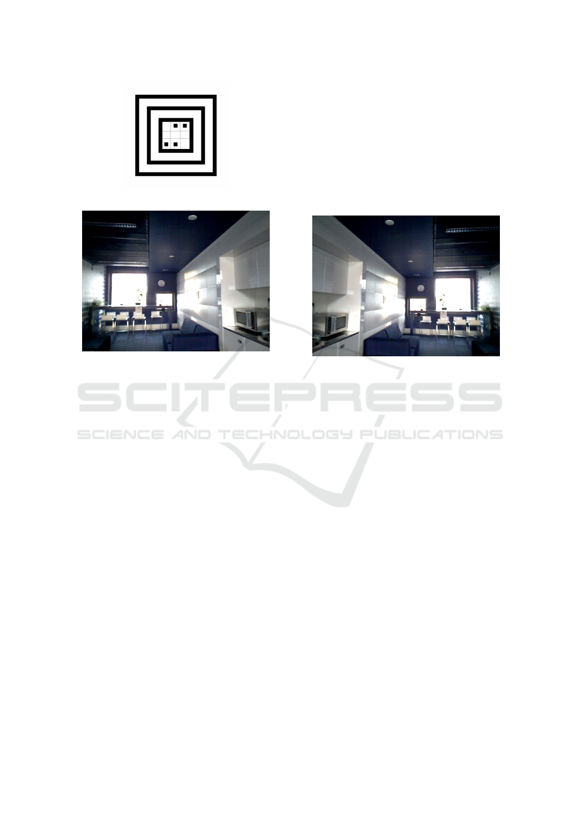
Figure 1: Visual Marker.

Figure 2: Dataset Scene Recognition Picture Example.

The ﬁnal step consists in using data augmentation

techniques, such as HSV light enchanting, as used by

(Dosovitskiy et al., 2014), to further increase the size

of the dataset up to 32,564 samples. For all the exper-

iments we use 80% of the dataset as training set, with

10% each as validation and testing sets. An example

image of this dataset can be seen in Figure 2.

2.2 Dataset for Location Recognition

After the considerations presented in Section 1, we

decided to create this dataset with explicit geometri-

cal variance properties. The dataset adds a new class

with all the images of our scene dataset that have been

ﬂipped. We use half of them as training, and the other

half as testing. We randomize the order of the pic-

tures to prevent the presence of only particular ﬂipped

classes in the training set while the other are in the

testing set. In this case we only use the non enhanced

images. This has been done to avoid too many similar

frames.

More precisely, the training set has all the original

images, divided in their respective classes, and a new

class is made, with a copy of the ﬂipped images. We

note that the test set has no original images, but only

ﬂipped ones. Half of these are in the training set, and

the other half form the whole test set. With this ex-

treme we can be sure to investigate how the different

methods can use necessary geometrical information.

This new dataset, with 11 classes, takes inspira-

tion from the one-vs-all approach similar to what has

been proposed in (Rifkin and Klautau, 2004). In fact,

this new class should be seen by the ANN as a noisy,

unique class. In order to do so, the network must ﬁnd

a way to distinguish this class from all the others: this

is only possible if the speciﬁc geometrical features are

considered.

An example of how we ﬂipped the pictures can be

seen by comparing Figure 2 and Figure 3.

Figure 3: Flipped Image Example.

3 METHODS

In this section we describe the different algorithms

that have been used for the experiments. Furthermore

we present a novel Deep Neural Network (DNN) ar-

chitecture that has been speciﬁcally designed for loca-

tion recognition in navigation tasks. We also present

the main considerations for developing our new archi-

tecture.

It is important to mention that all the experiments,

datasets and ANN architectures that are proposed are

contextualized with the creation of an optimal naviga-

tion system, based on visual information.

3.1 Histogram of SIFT Features

The ﬁrst approach that we evaluate is the Bag Of vi-

sual Words (BOW) based on the Scale Invariant Fea-

ture Transform. The Scale Invariant Feature Trans-

form, or SIFT (Lowe, 2004), has been used exten-

sively in the computer vision ﬁeld. The combination

of the SIFT key points descriptor algorithm, together

with the Bag Of visual Word (BOW) (Yang et al.,

2007), has performed very well in different scene

recognition tasks. This was the state of the art method

before the advent of Convolution Neural Networks.

The SIFT algorithm provides the detection of key

points and their relative descriptors. However, since

A Deep Convolutional Neural Network for Location Recognition and Geometry based Information

our dataset is generated from actual real world scenes,

it contains pictures with very little information. Ex-

amples of this information lack are white walls that

are not very informative in general, since they have

very few unique features.

As a consequence of this lack of information we

noticed that the SIFT detector only identiﬁes strong

key points on the VMs that are actually present in

the picture or frame. This results in a poor proper

generalization from the BOW representation of the

scenes and we therefore decided to not use the SIFT

detection algorithm. Instead, we use a dense grid of

key points over the pictures, and only rely on the key

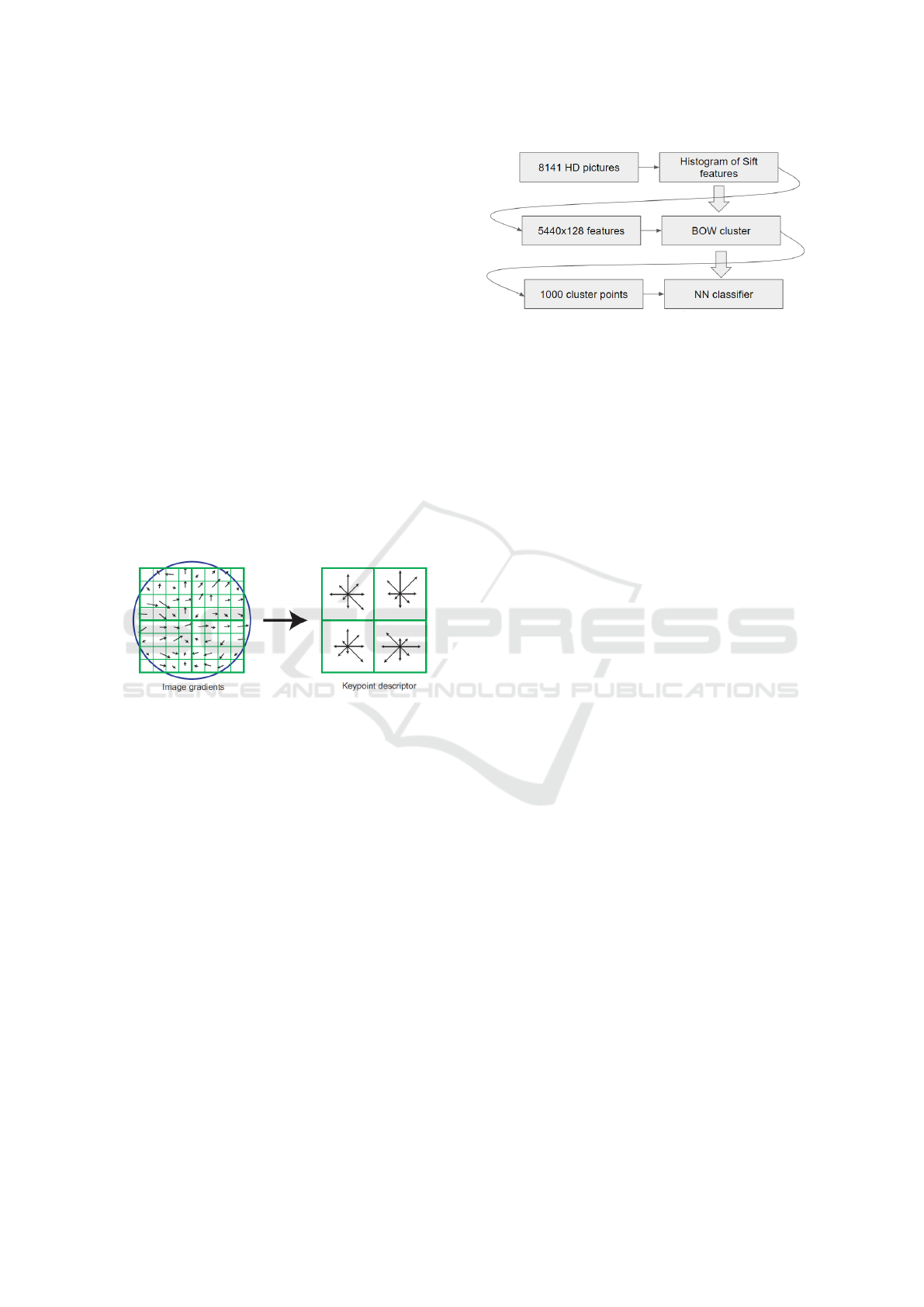
points descriptor algorithm. We take a key point ev-

ery 8 pixels, in both dimensions, and generate a total

amount of 5440 key points (160 × 34). For each key

point we consider a 16 × 16 pixel cell around it, and

divide it into four 4×4 cells. We then compute orien-

tations and magnitudes and order them in a histogram,

using 8 oriented bins. This generates, for every key

point, a 128 (4 · 4 · 8) features long vector. Figure 4

shows this approach.

Figure 4: SIFT Key Point Descriptors. Image taken from

(Lowe, 2004).

Since the neighbor cell shape is 16 × 16, and we

take a key point every 8 pixels, we have an overlap

for each descriptor. This overlap consists of 50% of

the size of a key point. This pipeline was also used in

(Marszałek et al., 2007).

Once we obtain 5440 × 128 features per picture,

we use the BOW clustering algorithm to reduce the

total number of features and create a visual codebook.

We train the BOW algorithm with a ﬁxed number of

cluster points, and use them to generate a histogram

of visual word occurrences. The length of this vector

is equal to the number of cluster points. The ﬁnal step

consists in using this vector as input for a neural net-

work (NN) used for the ﬁnal classiﬁcation task. We

show the full pipeline of the BOW approach in Figure

The NN architecture that we use is the following:

• Number of inputs: as many as the BOW cluster

points.

• Number of layers: input layer, one or two fully

connected hidden layers, output layer.

Figure 5: BOW pipeline.

• Activation function: the hidden layers use the

Leaky Rectiﬁed Linear Unit (LReLU). The output

layer uses the Softmax activation function.

• Number of outputs: as many as the VMs.

3.2 Convolutional Neural Networks

Convolutional Neural Networks (CNNs) are one of

the latest and most successful neural network archi-

tectures. This type of architecture started to become

extremely popular in 2012 (Krizhevsky et al., 2012),

and started to outperform all the other image recog-

nition methods, giving them a strong focus from the

scientiﬁc community. In particular CNNs perform re-

ally well with large datasets containing high resolu-

tion images. For these reasons they ﬁnd a vast utiliza-

tion in the computer vision ﬁeld.

Nowadays there exist many different types of

CNN architectures, that usually share the combina-

tion of Convolution Layer - Pooling Layer; making

this last type of layers vastly used. Pooling layers

were designed to reduce the size of the input, while

maintaining the key features in it. By applying a

pooling operation on the input, it can reduce the in-

put by a factor of 2, 3 or more while maintaining the

most prominent information. This is done by apply-

ing computational inexpensive operations like com-

puting the average or max. With these functions the

CNN can well represent the input information, and

drastically reduce its dimensionality. However, the

disadvantage is that precise geometrical information

is lost in this process. Performing a max operation

over a 3 × 3 grid, will hold on the most relevant fea-

tures in it, at the expense of the position of the fea-

tures. The deeper in the architecture this operation is

performed, the more geometrical precision is lost.

3.3 Inception Neural Network

The Inception Neural Network (INN) (Szegedy et al.,

2015) is a very promising novel CNN architecture.

The current state of the art in image classiﬁcation is

ICPRAM 2018 - 7th International Conference on Pattern Recognition Applications and Methods

achieved with the Inception V3 (Szegedy et al., 2016),

which is a tuned version of the original INN.

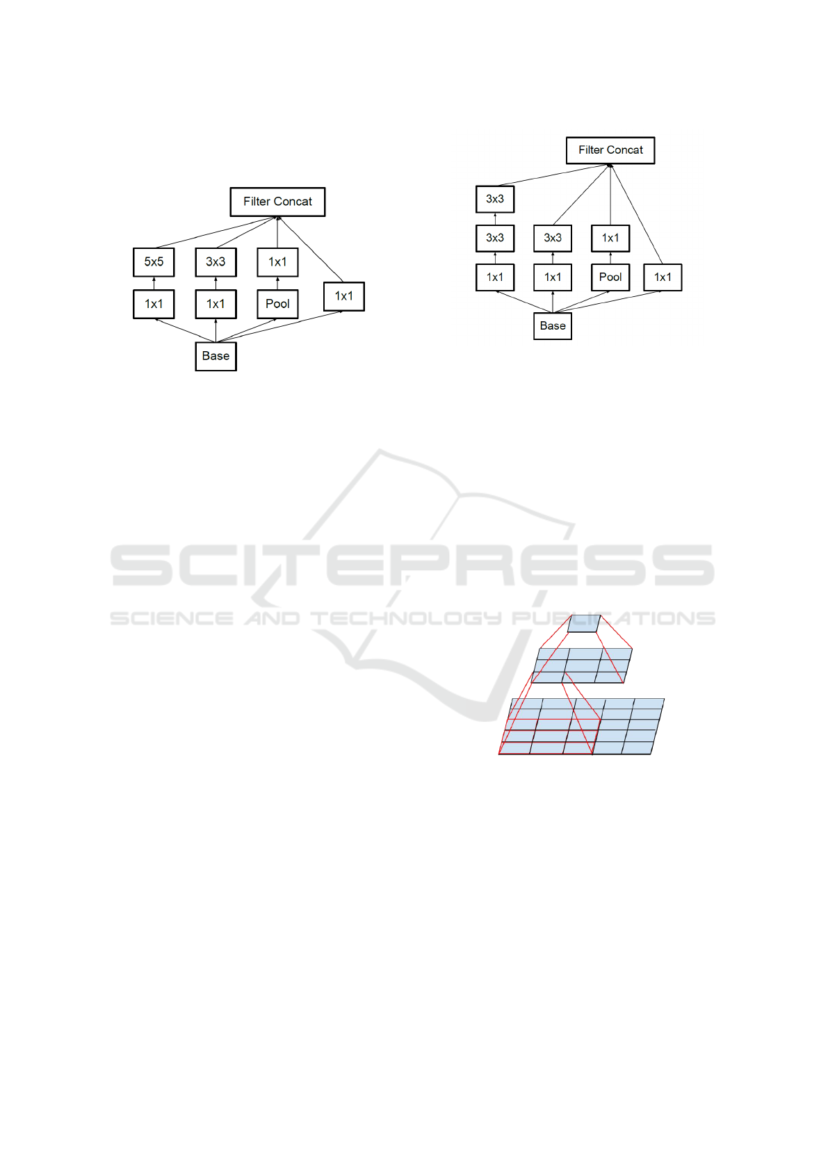
Figure 6: Inception Module. Image taken from (Szegedy

et al., 2015)

3.3.1 Inception Module

In the Inception Module, four different operations are

performed: a convolution with 5 × 5, 3 × 3 and 1 × 1

ﬁlters; and an average pooling operation. Also both

convolution operations are preceded by a 1 ×1 convo-

lution operation, in order to increase the depth of the

Inception Module. This architecture is represented in

Figure 6.

3.3.2 Inception V3

The Inception V3 (INN V3) architecture is a modi-

ﬁed version of the INN architecture. The main goal

of this architecture is to optimize as much as possible

deep neural network architectures. In fact the authors

achieved to create a deeper and wider structure, com-

pared to the original Inception module, without dras-

tically increasing the total number of weights. This

work takes inspiration from the Hebbian theory (Se-

jnowski and Tesauro, 1989), and follows the method

of (Arora et al., 2014). The key is to consider how

an optimal local sparse structure of a convolutional

neural network can be approximated and covered by

readily available dense components.

Figures 6 and 7 represent the original Inception

Module, and the adapted Inception V3 Module. It

can be seen that instead of the 5 × 5 convolution, two

consecutive 3 × 3 convolutions are used. This imme-

diately reduces the computational cost of the opera-

tions, given the smaller amount of weights to calcu-

late. In fact, a 5 × 5 convolution operation is com-

putationally more expensive than a 3 × 3 convolution

ﬁlter by a factor of 25/9 = 2.78. And while the 5 × 5

convolution ﬁlter can detect dependencies of signals

in further away units, if the same number of inputs is

Figure 7: Inception V3 Module. Image taken from

(Szegedy et al., 2016).

used for the ﬁrst 3 × 3 convolution, the second 3 × 3

convolution will reduce to 1 output maintaining intact

the 5 × 5 input/output ratio as shown in Figure 8.

This replacement reduces the computational cost,

while losing even more geometrical information.

When it is used for image classiﬁcation we can rely

on the translation invariance property: in order to de-

termine to which class an image belongs, it is only

needed to ﬁnd determinate features without consider-

ing where these are in the picture. As an example,

the system can determine if an image contains a dog,

regardless if it is on the left or right side of the picture.

Figure 8: Use of two 3 × 3 convolutions instead of 5 × 5.

Following the same idea, it is possible to exploit it

further, by considering to replace a 3 × 3 convolution

with a 3 × 1 and a 1 × 3 convolution in succession.

Again this will reduce the computational time, while

not losing meaningful information for object recog-

nition tasks thanks to the translation invariance prop-

erty.

Thanks to these adjustments the Inception V3 is

a 33 layers deep neural network, with a more than

acceptable number of weights of ≈ 1.3 millions. This

architecture is the current state of the art for image

classiﬁcation.

To test the performance of the Inception V3 archi-

A Deep Convolutional Neural Network for Location Recognition and Geometry based Information

tecture we use the pretrained network that is publicly

available on GitHub

. On the top of the architecture

we have added a fully connected layer of 250 hidden

units that is connected to the output layer consisting

of ten output units. The weights for these ﬁnal two

layers are the only parts of the network that we train

on the dataset.

3.4 New DNN Architecture

Considering the importance of geometrical informa-

tion in the navigation domain that we have presented

in section 1, we decided to build an ANN that would

never rely on geometrical invariance properties. As

already discussed, State of the Art methods vastly

use them. Furthermore, we also want to rely on

the effectiveness and efﬁciency of CNNs that are

very successful in the computer vision ﬁeld. In fact

since (Krizhevsky et al., 2012) they outperform all

other methods such as BOW for many different im-

age recognition problems.

The INN V3 heavily relies on geometrical in-

variance properties. This is because the architecture

makes extended use of e.g. pooling layers which

completely ignore the local geometry in their kernels

given their max or mean operations. If these layers are

applied in the deepest layers of the architecture, most

of the geometrical features get lost and are ignored

by the network. Besides pooling layers, other tech-

niques, such as the consecutive use of small convolu-

tion layers, extensively used in the INN V3, lose geo-

metrical properties. The use of two consecutive 3 × 3

convolution ﬁlters, instead of a 5 × 5 one; or even

more the use of 3 × 1 convolution followed by 1 × 3

convolution, heavily relies on the translation invari-

ance property. An extensive use of these techniques,

especially in the deeper levels of the architecture, has

a strong negative impact on the whole geometry of the

input.

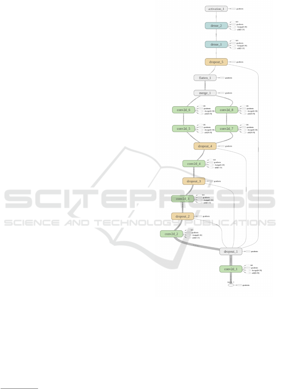
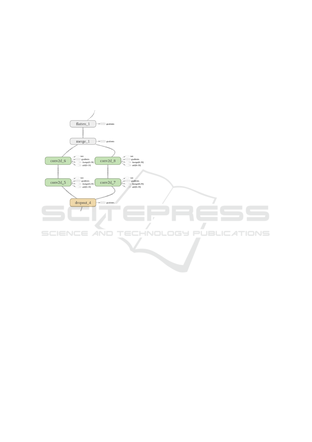
Here we present the architecture of our novel Nav-

DNN. The full structure can be seen in Figure 9. The

architecture consists of an input layer, followed by 4

convolution layers, an adapted Inception Module, a

hidden layer, and a ﬁnal output layer. The input pic-

tures have a 300 × 300 × 3 size, with the 3 ﬁnal chan-

nels corresponding to the RGB ones.

Hereafter we present into detail the parameters of

all the layers:

• Input: 300 × 300 × 3.

• Conv1: k=7; c=48; s=3; d=0.1; Ts=98x98x48.

• Conv2: k=9; c=32; s=2; d=0.1; Ts=45x45x32.

https://github.com/tensorﬂow/models/tree/master/inception

Figure 9: Nav-DNN architecture.

• Conv3: k=11; c=24; s=1; d=0.1; Ts=35x35x24.

• Conv4: k=22; c=16; s=1; d=0.1; Ts=14x14x16.

• Inception Layer: described in Figure 10

• Hidden: hidden units = 200.

• Output = 10.

Where k is the kernel size; c the number of chan-

nels; s the number of strides; d the dropout rate; and

T s the size of the output tensor size at each layer. The

Rectiﬁed Linear Unit (ReLU) activation function is

ICPRAM 2018 - 7th International Conference on Pattern Recognition Applications and Methods

used in all the convolution and hidden layers. A ﬁ-

nal softmax activation function is used for the output.

Figure 9 shows the just explained architecture.

As we can see from Figure 9 we use a modiﬁed

version of the Inception Module. We take inspiration

from the original one, with the difference that the one

that we create is able to maintain the geometrical in-

formation of the input. This difference is highlighted

in Figure 10.

Figure 10: Modiﬁed Inception Module.

We use in parallel 2 deep convolutions: on the left

a 1×1 kernel followed by a 3×3 one is used, while on

the right a 1×1 kernel followed by a 5 ×5 one is used.

We remove the pooling layer and all the weight opti-

mization techniques discussed in section 3.3.2. But

we still use the 1 × 1 convolution: in fact this allows

us to generate a deeper network while being at the

same time extremely cheap in terms of computational

resources.

Overall we maintained the beneﬁts of the origi-

nal inception layer: by placing this layer deep in our

architecture, we can have the beneﬁts of precise ge-

ometry relations, with the use of 3 × 3 convolutions

and more sparse geometry relations given by the 5×5

convolutions. Noticing that at this layer level the input

tensor has a shape of 14 ×14 × 16, so a 5×5 kernel is

able to ﬁnd relations in a geometrical space of more

than 1/3 of the original input, ≈ 100 × 100 pixels.

3.5 Training

The training procedures of the three methods pro-

posed slightly differ from each other given the diver-

sity of the algorithms.

The BOW algorithm, described in Section 3.1, has

been trained only on the original 8,141 HD pictures.

The training procedure took 72 hours. This is the rea-

son we decided to not use the enhanced dataset for

this algorithm, in order to not increase even more the

training time. We note that the clustering procedure

took 71.5 hours, while the training of the NN on top

of it took the remaining 30 minutes. Also for this

training the data set was split in 80% training, 10%

validation and test set. We trained the BOW only on

the Scene Recognition task.

The INN V3 algorithm, described in Section 3.3.2,

has been trained on a 32,564 pictures dataset for the

Scene Recognition task. This dataset is described in

Section 2.1, and we used 80% for training and 10%

for validating and testing. Since we used the pre-

trained INN V3, we only trained the last layer of the

network. In order to do this we computed the bottle-

neck tensor of every picture, then we used these for

the actual training of the last layer. Generating the

bottleneck tensors took 2.2 hours, while the training

of the last layer took less than 10 minutes. For the Lo-

cation Recognition Task, the total number of pictures

increased to 65,128. From these, 48,846 were used

for training and 16,282 were used for testing, as we

described in Section 2.2.

The Nav-DNN algorithm, described in Section

3.4, has been trained on 32,564 pictures for the Scene

Recognition task. This dataset is described in Section

2.1, and we used 80% for training and 10% for vali-

dating and testing. This algorithm took 1.5 hours to

train. For the Location Recognition Task, we used the

dataset described in Section 2.2.

4 RESULTS

In this section we present the results obtained on the

datasets. We will compare the performance of the

INN V3 with our novel Nav-DNN on the location

dataset described in section 2.2. We will also show

how geometrical information is intrinsic and used by

our DNN.

4.1 Results on Scenes Dataset

Here we report the results obtained on the dataset dis-

cussed in section 2.1. All the results can be seen in

Table 1. Here τ represents the computation time in

hours. The BOW approach obtained 88.5% accuracy

on the test set. These results were obtained with 1000

BOW cluster points, two hidden layers with 1000 and

500 hidden units, and a ReLU (Rectiﬁed Linear Unit)

activation function.

On the same dataset, the INN V3 outperforms the

BOW. The INN V3 obtained an accuracy of 100%.

A Deep Convolutional Neural Network for Location Recognition and Geometry based Information

Comparing the training time, the BOW trained for al-

most 3 days, while the INN V3 was trained for only 2

hours and 30 minutes. It is notable that the clustering

part of the BOW took the majority of the training time

since it was single threaded on the CPU, while the

INN V3 is pretrained except for the last hidden layer.

Most of the computation time was invested in creat-

ing the bottleneck output of the pretrained layers of

the INN V3. Nevertheless this last one, signiﬁcantly

outperforms the BOW.

Table 1: Scene Recognition Results.

Methods Val set Test set τ

BOW 89.7% 88.5% 72

INN V3 100% 100% 2.3

Nav-DNN 100% 98.7% 1.5

When we compare INN V3 with our architecture:

we can see that our network obtains an accuracy of

98.7% on the test set. While this is slightly worse

than the INN V3, it is important to verify how this

last architecture actually generalizes the pictures. In

particular to see if both DNN architecture generalize

the data in a meaningful way for a navigation system.

4.2 Results on Location Dataset

To verify this, we trained and tested both DNNs on the

location dataset described in section 2.2. The results

can be seen in Table 2.

Table 2: Location Recognition Results

NN architecture Correct Tricked Missed

INN V3 0% 97.43% 2.57%

Nav-DNN 99.7% 0% 0.3%

Here: Correct means the NN labeled the image

correctly; Tricked means the NN labeled the ﬂipped

image as the original one; and Missed means the NN

labeled the image as neither ﬂipped, neither as the

original image, but just as another class at random.

It is important to highlight that it is not possible

to distinguish a ﬂipped image from its original one by

only relying on the features. In fact, the two images

have exactly the same features, due to the way they

were constructed. The only successful approach to

distinguish the two pictures is to consider the geom-

etry of the image and the geometrical distribution of

the features.

These results perfectly show that it is possible to

create Deep Neural Networks, using convolution lay-

ers, that are able to maintain the geometrical property

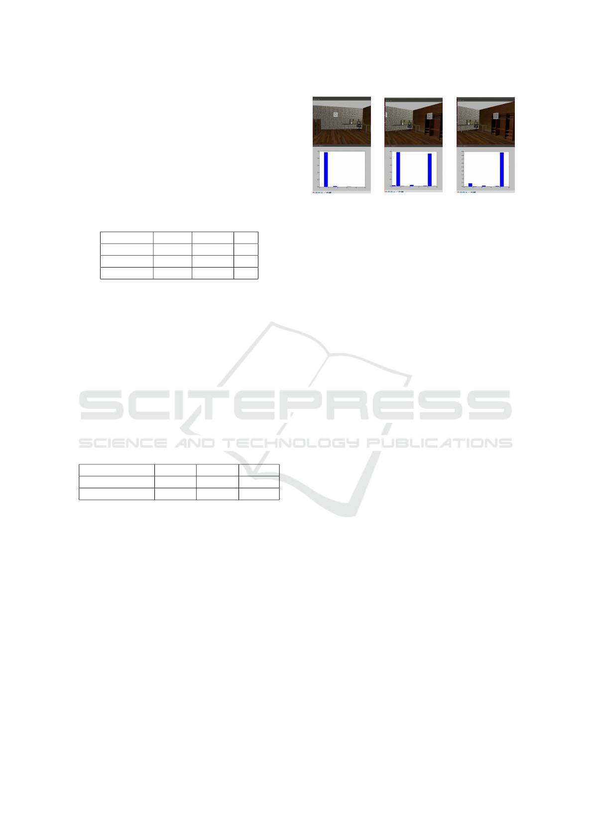
of the input. As can be seen from Figure 11, this is

essential for navigation tasks: identifying a speciﬁc

Figure 11: DNN output over camera rotation.

feature in the input is not enough, the position of this

feature is also essential.

Although we used real-word images for our ex-

periments, Figure 11 is constructed by using a sim-

ulator, Gazebo (Koenig and Howard, 2004), and the

new DNN we proposed. The top part of the pictures

show the point of view of the simulated robot, and the

bottom part shows the real output of the DNN as a

histogram of probabilities of the detected scene. This

process is in real time, with a live stream of frames

from the simulated camera, and real time classiﬁca-

tion of the DNN. In Figure 11 we show the most rel-

evant frame of the transition. From left to right, the

simulated robot turns right: we can see this move-

ment from the turning of the environment in the pic-

tures. This rotation changes the view from a scene to

the next one. Looking at the output of the DNN we

can see how we have a transition on scene probabili-

ties: this correlation between the physical rotation and

the transition of the probability from one scene to the

other is the clear sign of intrinsic geometrical infor-

mation derived from the DNN. This was completely

absent in the INN V3.

5 CONCLUSIONS AND FUTURE

WORK

In this paper we proposed a novel Deep Convolutional

Neural Network architecture that does not rely on the

geometrical invariance property. While using layers

like Pooling and weight optimization like the one used

in INN V3 greatly increase the performance of DNN

for scene recognition tasks, it is not the optimal choice

in every ﬁeld. Here we focused on navigation, where

geometry is essential for any navigation system. We

showed that it is possible to create high performing

DNNs that can also maintain the geometrical proper-

ties of the input, giving an intrinsic knowledge of the

geometry of the environment to the network itself.

Since the proposed DNN can be a key component

of a visual based navigation system, we focused on

experimenting on datasets which represent real world

ICPRAM 2018 - 7th International Conference on Pattern Recognition Applications and Methods

scenarios. The whole pipeline consists of an almost

autonomous way of generating labels, to create in a

fast way a dataset of the environment. This is used

to train the proposed DNN, which can generalize the

training data in a meaningful way: a direct correlation

between geometrical movement and the DNN output

probability. This is only possible when the DNN re-

lies on geometrical properties. It is also important to

notice that we experimented with removing the VMs

from the environment, and the DNN performances re-

main the same; but no extensive experiments were

performed with this focus.

To conclude, we show that it is possible to use

convolution layers to create deep architectures, while

maintaining all the geometrical properties of the data.

This can be applied in all the ﬁelds where the posi-

tion, or geometrical properties of the features are as

important as the features themselves.

Future Work. The new approach proposed in this

paper showed that is possible to use DNNs for ge-

ometrically based data. Moreover it can be applied

as the core localization subsystem for a visual based

navigation system. This would rely on the geometri-

cal properties of the real world environment to possi-

bly create a human like approach to navigation. If we

consider that humans are able to perfectly navigate in

any environment with solely visual information, then

the proposed approach would ﬁt the need of a human

like navigation system. To accomplish this, more con-

siderations and research needs to be done, focusing on

the system itself: the use of 3D cameras, stereoscopic

cameras and more.

On a more general level this approach shows po-

tential in applications where geometrical structure

matters. As an example we could consider FMRI

scans: these visual data are directly correlated to the

brain areas. Another example could be visual games:

from chess to Atari games. Given the ability of the

proposed DNN to rely on the positions of the fea-

tures and to generalize the geometrical properties of

the data, the possible beneﬁts are clear.

REFERENCES

Arora, S., Bhaskara, A., Ge, R., and Ma, T. (2014). Provable

bounds for learning some deep representations. In In-

ternational Conference on Machine Learning, pages

584–592.

Bonin-Font, F., Ortiz, A., and Oliver, G. (2008). Visual

navigation for mobile robots: A survey. Journal of

intelligent and robotic systems, 53(3):263.

Dosovitskiy, A., Springenberg, J. T., Riedmiller, M., and

Brox, T. (2014). Discriminative unsupervised fea-

ture learning with convolutional neural networks. In

Advances in Neural Information Processing Systems,

pages 766–774.

Elfes, A. (1987). Sonar-based real-world mapping and nav-

igation. IEEE Journal on Robotics and Automation,

3(3):249–265.

Everett, H. R. and Gage, D. W. (1999). From labo-

ratory to warehouse: Security robots meet the real

world. The International Journal of Robotics Re-

search, 18(7):760–768.

Floreano, D. and Wood, R. J. (2015). Science, technology

and the future of small autonomous drones. Nature,

521(7553):460.

Guivant, J., Nebot, E., and Baiker, S. (2000). Autonomous

navigation and map building using laser range sensors

in outdoor applications. Journal of robotic systems,

17(10):565–583.

Koenig, N. and Howard, A. (2004). Design and use

paradigms for gazebo, an open-source multi-robot

simulator. In Intelligent Robots and Systems. Pro-

ceedings. 2004 IEEE/RSJ International Conference

on, volume 3, pages 2149–2154.

Krizhevsky, A., Sutskever, I., and Hinton, G. E. (2012). Im-

agenet classiﬁcation with deep convolutional neural

networks. In Advances in neural information process-

ing systems, pages 1097–1105.

LeCun, Y., Bengio, Y., and Hinton, G. (2015). Deep learn-

ing. Nature, 521(7553):436–444.

Levinson, J., Askeland, J., Becker, J., Dolson, J., Held, D.,

Kammel, S., Kolter, J. Z., Langer, D., Pink, O., Pratt,

V., et al. (2011). Towards fully autonomous driving:

Systems and algorithms. In Intelligent Vehicles Sym-

posium (IV), 2011 IEEE, pages 163–168. IEEE.

Lowe, D. G. (2004). Distinctive image features from scale-

invariant keypoints. International journal of computer

vision, 60(2):91–110.

Marszałek, M., Schmid, C., Harzallah, H., and Van De Wei-

jer, J. (2007). Learning object representations for vi-

sual object class recognition. In Visual Recognition

Challenge workshop, in conjunction with ICCV.

Rifkin, R. and Klautau, A. (2004). In defense of one-vs-all

classiﬁcation. Journal of machine learning research,

5(Jan):101–141.

Sejnowski, T. J. and Tesauro, G. (1989). The Hebb rule for

synaptic plasticity: algorithms and implementations.

Neural models of plasticity: Experimental and theo-

retical approaches, pages 94–103.

Sukkarieh, S., Nebot, E. M., and Durrant-Whyte, H. F.

(1999). A high integrity imu/gps navigation loop for

autonomous land vehicle applications. IEEE Transac-

tions on Robotics and Automation, 15(3):572–578.

Szegedy, C., Liu, W., Jia, Y., Sermanet, P., Reed, S.,

Anguelov, D., Erhan, D., Vanhoucke, V., and Rabi-

novich, A. (2015). Going deeper with convolutions.

In Proceedings of the IEEE conference on computer

vision and pattern recognition, pages 1–9.

Szegedy, C., Vanhoucke, V., Ioffe, S., Shlens, J., and Wo-

jna, Z. (2016). Rethinking the inception architecture

for computer vision. In Proceedings of the IEEE Con-

ference on Computer Vision and Pattern Recognition,

pages 2818–2826.

A Deep Convolutional Neural Network for Location Recognition and Geometry based Information

Yang, J., Jiang, Y.-G., Hauptmann, A. G., and Ngo, C.-W.

(2007). Evaluating bag-of-visual-words representa-

tions in scene classiﬁcation. In Proceedings of the

international workshop on multimedia information re-

trieval, pages 197–206. ACM.

ICPRAM 2018 - 7th International Conference on Pattern Recognition Applications and Methods