Multiple Sclerosis Lesion Segmentation using Improved Convolutional

Neural Networks

Erol Kazancli

1,2

, Vesna Prchkovska

, Paulo Rodrigues

, Pablo Villoslada

and Laura Igual

Department of Mathematics and Computer Science, Universitat de Barcelona,

Gran Via de les Corts Catalanes, 585, 08007 Barcelona, Spain

DAMA-UPC, Universitat Polit

ecnica de Catalunya, C. Jordi Girona, 1-3, 08034 Barcelona, Spain

Mint Labs Inc. 241 A Street Suite 300, 02210 Boston, MA, U.S.A.

Center of Neuroimmunology, Institut d’Investigacions Biomediques August Pi Sunyer (IDIBAPS),

Villarroel, 170, 08036 Barcelona, Spain

Keywords:

Multiple Sclerosis Lesion Segmentation, Deep Learning, Convolutional Neural Networks.

Abstract:

The Multiple Sclerosis (MS) lesion segmentation is critical for the diagnosis, treatment and follow-up of

the MS patients. Nowadays, the MS lesion segmentation in Magnetic Resonance Image (MRI) is a time-

consuming manual process carried out by medical experts, which is subject to intra- and inter- expert variabi-

lity. Machine learning methods including Deep Learning has been applied to this problem, obtaining solutions

that outperformed other conventional automatic methods. Deep Learning methods have especially turned out

to be promising, attaining human expert performance levels. Our aim is to develop a fully automatic met-

hod that will help experts in their task and reduce the necessary time and effort in the process. In this paper,

we propose a new approach based on Convolutional Neural Networks (CNN) to the MS lesion segmentation

problem. We study different CNN approaches and compare their segmentation performance. We obtain an

average dice score of 57.5% and a true positive rate of 59.7% for a real dataset of 59 patients with a speciﬁc

CNN approach, outperforming the other CNN approaches and a commonly used automatic tool for MS lesion

segmentation.

1 INTRODUCTION

Multiple Sclerosis (MS) is a chronic neurological di-

sease that afﬂicts especially the young population be-

tween the ages 20 and 50. It affects 2.3 million pe-

ople worldwide and can cause symptoms such as loss

of vision, loss of balance, fatigue, memory and con-

centration problems, among others. It remains a very

challenging disease to diagnose and treat, due to its

variability in its clinical expression (National MS So-

ciety, 2017). MS is characterized by lesions throug-

hout the brain that are caused by the loss of mye-

lin sheath around neurons in the brain, which is also

known as demyelination. The lesions are visible in se-

veral modalities of Magnetic Resonance Image (MRI)

with different contrasts. The number and the total vo-

lume of MS lesions are indicative of the disease stage

and are used to track disease progression.

The accurate segmentation of lesions in MRI is

important for the accurate diagnosis, adequate treat-

ment development and patient follow-up of the MS

disease. Manual segmentation of MS lesions by ex-

perts is the most commonly used technique and is still

considered to produce the most accurate results alt-

hough it suffers from many complications. First of

all, it is subject to intra- and inter- expert variability,

which means there are signiﬁcant differences between

two segmentations performed by two different experts

(due to slightly varying deﬁnitions) or by the same

expert at different times (due to fatigue or similar fac-

tors). Secondly there is a shortage of adequately trai-

ned experts given the huge amount of segmentation

need. Thirdly, the segmentation task requires valuable

expert time and concentration, which could ideally be

dedicated to other tasks. These drawbacks make it

necessary and desirable to develop a semi-automatic

segmentation method that would assist experts in the

task with a reduced amount of time and intra- inter-

expert variability or, in the ideal case, a fully auto-

matic segmentation method which would obviate the

need for experts and produce accurate/reproducible

results.

260

Kazancli, E., Prchkovska, V., Rodrigues, P., Villoslada, P. and Igual, L.

Multiple Sclerosis Lesion Segmentation using Improved Convolutional Neural Networks.

DOI: 10.5220/0006540902600269

In Proceedings of the 13th International Joint Conference on Computer Vision, Imaging and Computer Graphics Theory and Applications (VISIGRAPP 2018) - Volume 4: VISAPP, pages

260-269

ISBN: 978-989-758-290-5

Several methods previously presented in the lite-

rature resort to machine learning approaches. Some

methods use supervised approaches with hand-crafted

features or learned representations and some other

methods use unsupervised approaches like clustering

which aim to detect lesion voxels as outliers. Ex-

amples of supervised models used in MS segmenta-

tion tasks are k-nearest neighbour methods, artiﬁcial

neural networks, random decision forests and baye-

sian frameworks among others (Garcia-Lorenzo et al.,

2013). Examples of unsupervised models are fuzzy c-

means or Gaussian mixture models with expectation

maximization (EM) (Garcia-Lorenzo et al., 2013).

Unsupervised models suffer from non-uniformity in

the image intensities and lesion intensities since this

variability cannot be captured by a single global mo-

del (Havaei, 2016). In this respect supervised met-

hods present an advantage, potentially being able to

capture this variability with the appropriate choice of

training set or features.

Recently, Deep Learning (DL) has been very

successful in the Computer Vision area, achieving

improvements in accuracies sometimes as high as

30% (Plis et al., 2014). The main strength in DL,

also differentiating it from other machine learning

methods, is its automatic feature extraction capability.

Normally, raw data has to be processed automatically

or manually to extract meaningful and useful featu-

res through a process commonly known as ”feature

engineering”. This process requires time and careful

analysis, and includes subjectivity, which might bias

the results or produce erroneous results. However,

in DL, the feature extraction is data-driven using an

appropriate loss function and learning algorithm for

Deep Neural Networks, which removes the subjecti-

vity, randomness and expert knowledge to a certain

degree. Moreover, the features obtained are hierarchi-

cal, each network layer producing more abstract fea-

tures using the less abstract features obtained in the

previous layer. Thus feature extraction is carried out

step-by- step, which is likelier to produce more com-

plex and useful features. Another strength of DL is

its ability to represent very complex functions, which

might also be considered as its drawback since it is

prone to easily over-ﬁt. However, the over-ﬁtting can

be prevented with the correct guidance and regulariza-

tion methods. DL methods are also robust to outliers,

which is very common in neuroimaging data (Good-

fellow et al., 2016), (Bengio, 2012) and (Deep Lear-

ning, 2017).

Previous work on MS lesion segmentation with

DL is generally developed using voxelwise classiﬁca-

tion (lesion vs. normal) and is done on 2D/3D patches

centered on the voxel of interest to obtain a complete

segmentation of the whole brain (Greenspan et al.,

2016). There are also some studies considering the

whole image as input and performing a segmentation

in a single step as in (Brosch et al., 2015) and (Brosch

et al., 2016). In some methods global context is pro-

vided to the network, in addition to the local con-

text, to give more information about the nature of a

voxel (Ghafoorian et al., 2017). Convolutional Neu-

ral Networks (CNNs) are commonly used as part of

the architecture due to their strong feature extraction

capabilities dealing with images (Vaidya et al., 2015),

while Restricted Boltzmann Machines (RBMs) and

Auto-encoders are generally exploited to obtain a

good initialization of the network, which might affect

the ultimate performance, as shown in (Brosch et al.,

2015) and (Brosch et al., 2016).

In this paper, we propose a MS lesion segmen-

tation method based on a voxelwise classiﬁcation on

MRI with DL using a combination of different appro-

aches presented in the literature together with our own

contributions. We explore a new sub-sampling met-

hod to improve the learning process and develop a

new Convolutional Neural Networks (CNN) approach

to achieve better performance results. The aim of this

study is to achieve a method that will surpass the per-

formance of existing methods in helping the experts

in the MS lesion segmentation work and even make

their interruption minimal. We compare different ap-

proaches with DL so far applied to MS Segmentation.

2 METHODOLOGY

In this section, we present our strategies for data

pre-processing, sub-sampling of the training set, de-

signing the CNN architecture and developing diffe-

rent approaches to improve the segmentation perfor-

mance.

2.1 Data Pre-processing

We have, at our disposal, T1 and T2 MRI modali-

ties, tissue segmentation and manual lesion segmenta-

tions of 59 subjects from Hospital Cl

ınic (Barcelona).

The tissue segmentation was performed by Freesurfer

v.5.3.0 toolbox (Freesurfer, 2013). The manual seg-

mentation was performed by an expert / two experts

from Hospital Cl

ınic team. The voxel resolution of

the MRIs is 0.86mm x 0.86mm x 0.86mm and the

image size is 208 x 256 x 256. As a pre-processing of

the MRI images we apply skull stripping, bias-ﬁeld

correction, tissue-segmentation and co-registration.

Additionally we apply 0-mean unit-variance normali-

Multiple Sclerosis Lesion Segmentation using Improved Convolutional Neural Networks

261

zation to the data. For this process we use the Scikit-

Learn’s preprocessing package (Scikit-Learn, 2010).

2.2 Sub-sampling Strategy

We pose the segmentation problem as a voxelwise

classiﬁcation throughout the MRI image; therefore,

by a sample we mean a 3D patch centered on the voxel

of interest (to be classiﬁed). Initially we consider pa-

tches of size 11x11x11. A positive sample is such

a patch centered on a lesion voxel, while a negative

sample is a patch centered on a non-lesion voxel.

The data comes with a big imbalance of positive-

negative samples; negative samples greatly outnum-

bering the positive ones, because the lesion regions

generally make up a very small proportion of the

whole brain. To overcome this problem in the trai-

ning set, we take all the positive samples and select

as many negative samples using two different appro-

aches: random sampling and sampling around the le-

sions.

By random sampling we mean choosing negative

samples randomly throughout the brain, without ta-

king into account its location. By sampling around

lesions we mean taking negative samples very close

to the lesion areas. The latter approach produced bet-

ter results in the initial experiments therefore we kept

to this approach in the ﬁnal experiments. This might

be due to the fact that in the random sampling met-

hod, the selected negative samples are very similar to

each other and does not represent the diversity of the

negative samples. However, when we select the nega-

tive samples around the lesions, we add more variety

and harder cases to the training set. In addition, we

avoid the negative examples very close to (2-voxels)

lesion regions, since these voxels may be in reality le-

sion voxels although they were not labeled as such by

the expert.

Finally, it is important to note that we select the

samples from white and gray matter although the stu-

dies so far generally chose their data from only white

matter since the probability to have a lesion in the

white matter is far greater than having it in the gray

matter.

2.3 Patch-based Classiﬁcation using

CNN

Our initial CNN architecture is based on the

study (Vaidya et al., 2015) with several differences.

We use a simple CNN architecture with two convolu-

tional layers and one fully connected layer. The pa-

tches are 3D cubes centered on the voxel of interest,

which are obtained from T1 and T2 images. The ﬁrst

convolutional layer uses 60 kernels of size 4x4x4 with

a stride value of 1 and no padding. This layer is fol-

lowed by an average pooling layer that takes 2x2x2

patches of the output generated in the previous layer

and produces an average for each patch. The stride

value for average pooling is 2. The second convoluti-

onal layer consists of 60 kernels of size 3x3x3 with

a stride value of 1 and no padding. After this se-

cond layer of convolutions we use average pooling of

2x2x2 patches with a stride value of 2 and followed

by a fully connected layer. This layer consists of 200

hidden units that are fully connected to the output of

the previous layer.

In the study (Vaidya et al., 2015) authors use 3 mo-

dalities T1, T2, and FLAIR, but we use only two, T1

and T2 since we do not have the FLAIR modality for

our patients. The patch size they use is 19x19x19 but

since our images have nearly half the resolution of the

images used in the study we choose our initial patch

size as 11x11x11. They consider different modalities

as input channels and start from 4D data. We chose to

start with separate branches from different modalities

and merge them at the fully-connected layer since our

experiments show improvements with this approach.

Also our subsampling method which was explained in

the previous section, differs from theirs.

For the convolutional layers and fully connected

layer ReLU (Rectiﬁed Linear Unit) is used as acti-

vation function. The output layer is a softmax layer

of two units, which produces a probability for the two

classes, which are lesion and non-lesion for the center

voxel. The class with a higher probability is the deci-

sion class produced. To compute gradients and guide

the training of the network cross-entropy loss function

is used. We use mini-batch gradient descent with a

batch size of 128 for each training step. To adjust

the convergence speed of the algorithm, an adaptive

learning method, namely Adam (Adaptive Moment

Estimation) is used which adapts the momentum and

learning rate throughout the training. At the convolu-

tional layers, batch normalization is applied, which is

known to lead to faster convergence and which serves

as a type of regularization method. We apply dropout

to the fully connected layer to add further regulariza-

tion. The number of epochs is set experimentally. An

scheme of the proposed architecture can be seen in

Figure 1.

2.4 Improvements of the Original

Model

Starting from the ﬁrst model described above, we test

several approaches with different experimental set-

tings and improvements of the original approach: le-

VISAPP 2018 - International Conference on Computer Vision Theory and Applications

262

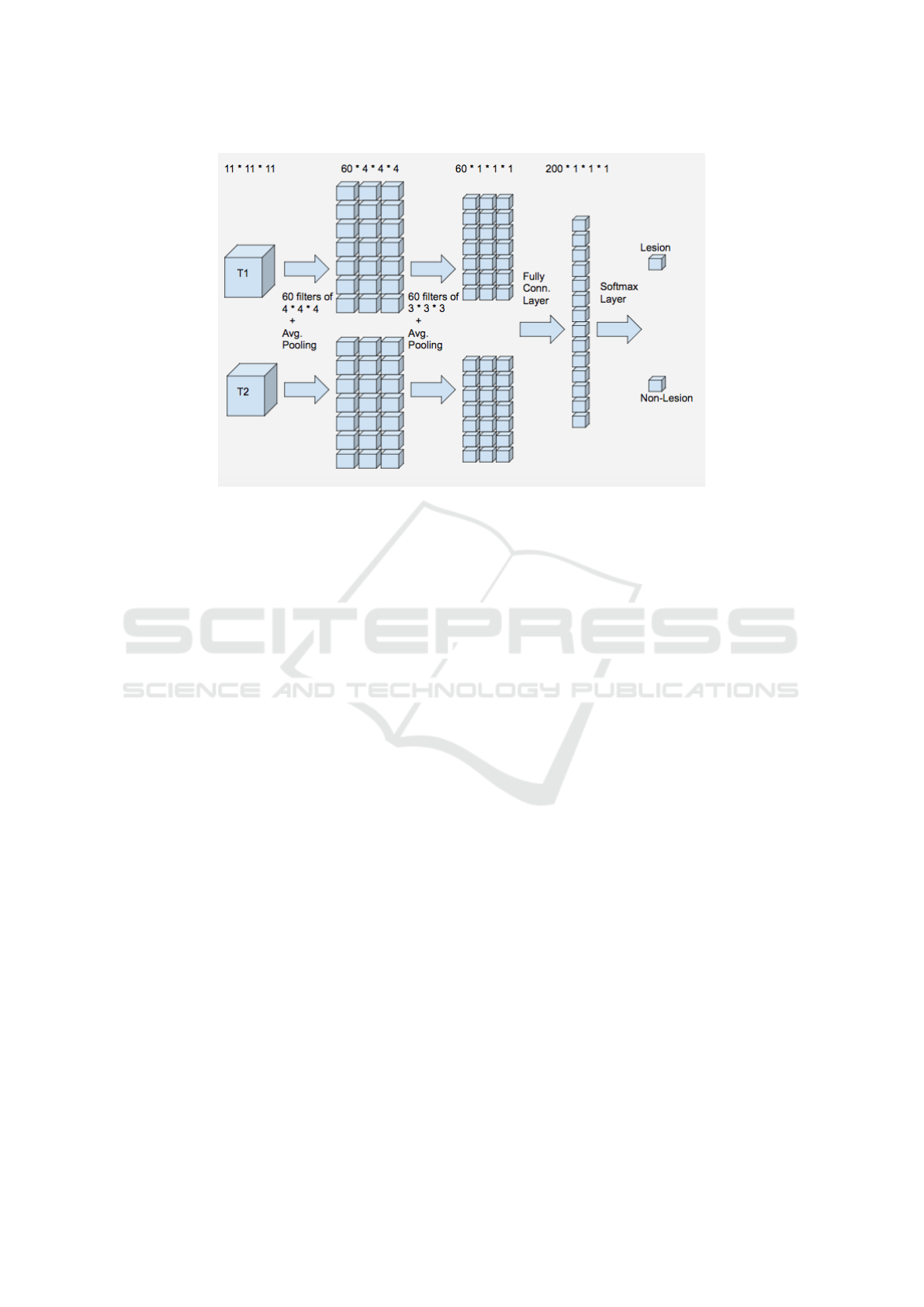
Figure 1: Proposed CNN Architecture.

sion location information, multi-class classiﬁcation

and cascade approach.

Lesion Location Information. As a second appro-

ach, we add the lesion location information to the fe-

ature set to test if it improves the results. We think

this information might be useful since the probability

of having a lesion in certain regions of the brain might

show differences. For this approach we store the x, y,

z coordinates of each patch, we normalize them and

add these features at the fully connected layer. The

additional computational cost by adding these 3 fea-

tures is negligible for training and testing.

Patch Size. As the third approach, we increase the

patch size from 11x11x11 to 19x19x19 to see if gi-

ving more information of the context improves the

results. Note that increasing the patch-size increases

the number of initial features cubically. This means

increasing the computational cost substantially. We

keep the location information for this approach and

further approaches.

Cascade. Up to this point, the main problem in the

obtained results of our approaches is the high num-

ber of false positives obtained. Even though true ne-

gative rates reached levels of 96% the resulting seg-

mentation contained a high number of false positives,

even surpassing the number of true lesion voxels, due

to the high number of non-lesion voxels in the brain

compared to the lesion voxels. This is undesirable for

an automatic segmentation technique since the human

expert will need to discard these false positives, which

might even make the automatic segmentation useless.

The next approach focuses on decreasing these false

positives.

In the fourth approach, we implement two CNNs

in a cascade fashion as proposed in the study of (Val-

verde et al., 2017). We implement a CNN as explai-

ned before (in the second approach, with 11x11x11

patch size and location information) and obtain a ﬁrst

model. With this model, we segment all the training

subjects automatically, which are used in the selection

of training samples for the second stage. For the se-

cond model, we use exactly the same architecture as

in the ﬁrst stage but the sampling method differs. For

positive samples, we choose all the lesion voxels; For

the negative samples, we choose as many non-lesion

voxels in such a fashion that half of this number co-

mes from the false positives, which were wrongly

classiﬁed negative samples in the ﬁrst stage, and the

other half comes from the true negatives from the ﬁrst

stage segmentation results. The reason to choose the

false positives is to be able to remove these false po-

sitives in the second stage and the reason to choose

from true negatives is to prevent the model to forget

the knowledge obtained in the ﬁrst model. In the ori-

ginal study negative samples are only selected from

the false negatives, which in our case performed far

from desired. The second stage model is thus trained

with the samples selected as just explained. In the tes-

ting stage, an initial segmentation is obtained using

the ﬁrst CNN model. The candidate lesions obtained

from the ﬁrst model are fed into the second model and

a ﬁnal segmentation is obtained with the resulting po-

sitives of the second model. The computational cost

to the training of this model is more than twice the

cost of a one-stage model, since it also includes the

evaluation of all the training samples. However, once

Multiple Sclerosis Lesion Segmentation using Improved Convolutional Neural Networks

263

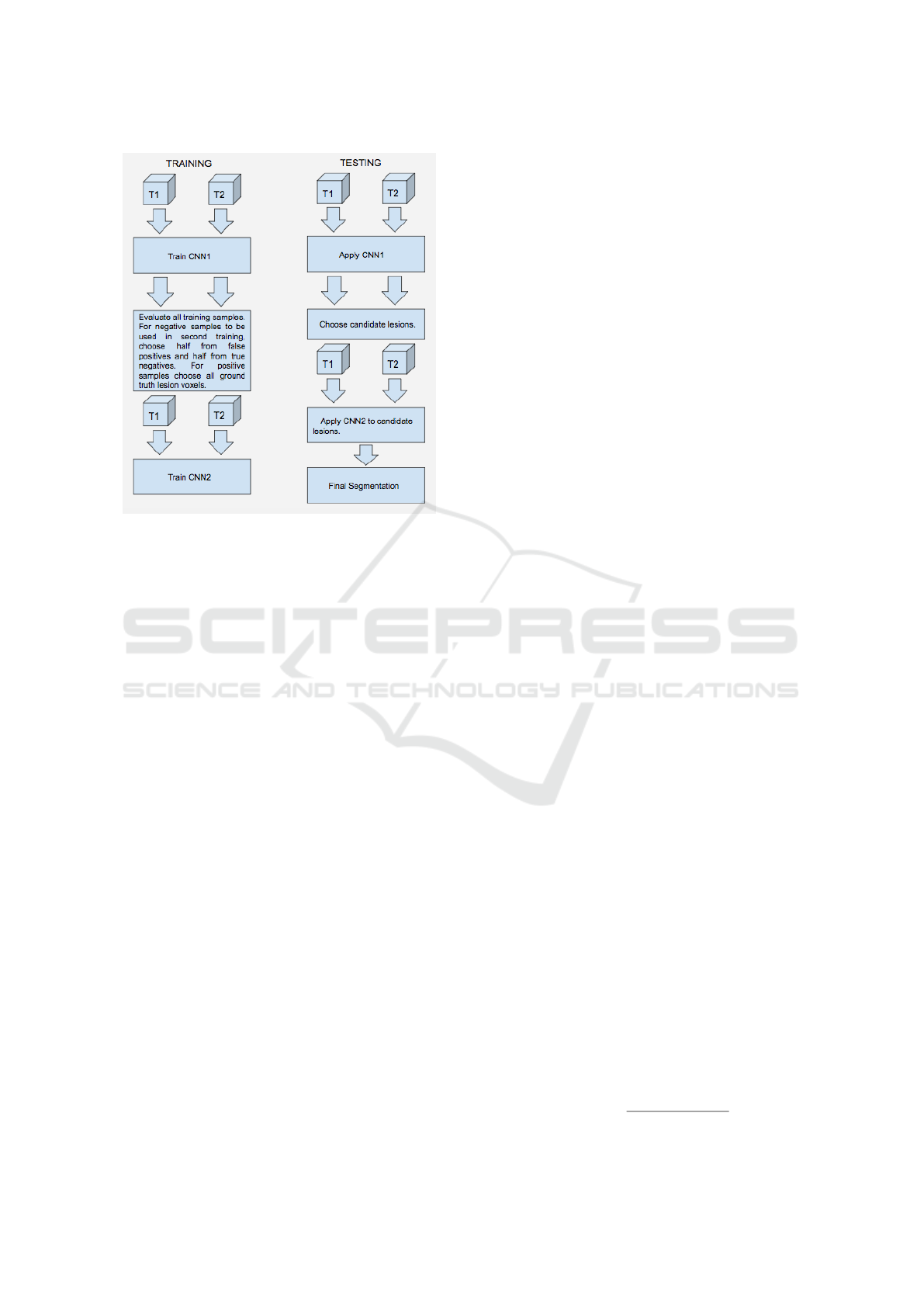
Figure 2: Two stage training and testing - Cascade.

the training is obtained the computational cost for tes-

ting does not double since the samples evaluated in

the second stage are a very small proportion of the

whole sample set. Figure 2 illustrates the cascade ap-

proach.

With the cascade implementation we should re-

duce the number of false positives at the cost of losing

also some of the true positives, but hopefully the gain

is considerably higher than the loss.

Multi-class Classiﬁcation Problem. We realize that

there is a difference in the accuracy rates between the

region along the border of a lesion and the region far-

from a lesion border. This observation brought to our

minds to try ﬁrst a 4-class model and subsequently

a 3-class model. For the ﬁfth approach, we incre-

ase the number of classes from 2 (lesion, non-lesion)

to 4 (lesion interior, lesion border, non-lesion border,

non-lesion interior) during training to try to reduce

the false positive rate. During testing, we merge the 4

classes back to 2 classes.

The problem with the 4-class model is that the

number of lesion interior voxels is quite low com-

pared to the number of other classes and to balance

the training set we have to decrease the number of

samples substantially. This is something undesirable,

thus we consider lesion voxels as one class, and di-

vide the non-lesion voxels into two classes, which are

border non-lesion, interior non-lesion. Thus, for the

sixth approach, we consider 3 classes (lesion, border

non-lesion, interior non-lesion).

As a last step, we test the cascade implementation

with this 3-class model as a seventh approach. This is

the exact same cascade approach explained before in

the fourth approach, but with 3 classes instead of 2.

2.5 Technical Speciﬁcations

In order to develop our DL approaches we use an EC2

instance of type p2.xlarge of Amazon Web Services.

This is a cloud service of Amazon with GPU that pro-

vides high computational power for computationally

intensive processes such as DL (Amazon, 2017). It

also comes with an execution environment that con-

tains DL frameworks such as Tensorﬂow, Caffe, The-

ano, Torch, etc. We use Python as a programming

language and Tensorﬂow as a DL framework to im-

plement and run our DL algorithms. We also use

cloud storage provided by Amazon to store our trai-

ning samples. We handle the neuroimaging ﬁles in

the NIfTI-1 format with the Nibabel library of py-

thon (Nibabel, 2017).

3 EXPERIMENTS AND RESULTS

In this section, we describe the validation strategy

(data distribution and validation measures), the expe-

riments and obtained results.

3.1 Validation Strategy

As we already described in section 2.1, the ground-

truth (GT) is made by T1 and T2 MRI modalities,

tissue segmentation and manual lesion segmentations

from 59 subjects.

For the distribution of data to train, validation and

test, we allocate 45 subjects to train, 5 subjects to va-

lidation and 9 subjects to test data. We use valida-

tion accuracy to determine the number of epochs with

which to train the networks. In the experiments, af-

ter 60 epochs the validation accuracy did not improve

and even started to drop, for this reason we decided to

stick to this number for the training of our networks,

to prevent over-ﬁtting.

As validation measures we consider four different

measures detailed next.

Dice Similarity Coefﬁcient (DSC) is a statistical

overlapping measure that quantiﬁes the similarity be-

tween two segmentations. This measure is between 0

and 1; 0 meaning no similarity and 1 meaning a per-

fect match between segmentations. We compute it as

a percentage as follows.

DSC = 100

2T P

2T P + FP + FN

VISAPP 2018 - International Conference on Computer Vision Theory and Applications

264

where TP is the number of True Positives, FP is the

number of False Positives, and FN is the number of

False Negatives.

True Positive Rate (TPR) is the percentage of the le-

sion voxels with respect to the total GT lesion voxels,

which is also called the sensitivity. This measure is

between 0 and 1, and the higher the better although

it has to be considered together with other measures

for the quality of the segmentation. We express it as a

percentage.

T PR = 100

T P

#LV GT

where #LVGT is the number of lesion voxels in the

GT.

False Discovery Rate (FDR) is the percentage of

false positive voxels with respect to the output seg-

mentation performed by the method. The measure is

between 0 and 1, and low values are desired. We ex-

press it as a percentage.

FDR = 100

#LV f ound

where #LV found is the number of lesion voxels de-

tected by the method.

Volume Difference (VD) is the percentage of the ab-

solute difference between the GT lesion volume and

the volume of the lesions found by the automatic met-

hod with respect to the GT lesion volume. This me-

asure does not give information about the overlap of

the two segmentations but gives an idea about the re-

lative volumes. The minimum and the ideal value for

this measure is 0 but there is no maximum for this me-

asure. 0 value means the lesion volumes in the met-

hod segmentation and the GT are the same in size,

although it might mot mean a perfect overlap. We ex-

press it as a percentage.

V D = 100

k#LV f ound − #LV GT k

#LV GT

Moreover, we also consider the computation of

#CC lesion GT: The number of connected compo-

nents (CCs) in the GT segmentation; #CC lesion

found: The number of connected components found;

and #CC lesion coincided: The number of connected

components in the GT that has some overlap with

the connected components in the method segmen-

tation. Note this might be bigger that the number

of connected components found since one CC found

can coincide with multiple CCs in the ground truth.

A Connected Component (CC) can be deﬁned as a

group of lesion voxels connected with each other and

it can be of different sizes.

3.2 Results

Tables 1 and 2 contain the results of the seven appro-

aches considered in the paper together with LST ap-

proach. As can be seen the ﬁnal model, which is the

3 class model with cascade have the best performance

in all the measures except the TPR. The decrease in

the TPR is understandable, since as we removed the

FP we also had to sacriﬁce some TP; although in com-

parison it is very small in number. The best model

also surpassed the LST method in all the measures in-

cluding the TPR.

Note that values in Table 2 have to be compared

with # Lesion Voxels in GT (#LV GT) which is 11573

± 9873 and # Lesion CC in GT (#LCC GT) which is

125.6 ± 61.4. As can be seen, the detected number of

lesions is closest to the real number with the 3-class

cascade model, which means the false negatives have

substantially been eliminated. Also with this model,

around 102 CCs are detected, and there is some over-

lap with 72 of the LCCs in the GT, which is the hig-

hest proportion among the models. Although there

are other models with higher LCC coincided with the

GT, these models have an exorbitantly high number of

LCCs found, the majority of which are false detecti-

ons.

Besides analyzing the quantitative results and to

better understand the behavior of the segmentation al-

gorithm on the MRI images, we qualitatively inspect

the results in Figure 3 and Figure 4.

Figure 3 shows the results of the best model in ex-

ample images from 4 subjects of the test set. The ma-

nual segmentation or TP are shown in dark blue, the

FP in light blues, and the FN in pink. As can be seen

from the ﬁgure, there is detection around the GT seg-

mentation for most of the lesions and there is a high

amount of overlap but there are also differences. The

differences can be partly due to the subjective nature

of manual MS segmentation or difﬁculty in obtaining

the real borders, even by a human expert.

Figure 4, which is an up-close version of a re-

gion from Figure 3. It shows the T1 image (left), the

T2 image (middle) and segmentation result (right) of

the same region. As can be seen from the ﬁgure, the

manual segmentation is more conservative while our

model is over-segmenting a region as lesion if there

is a corresponding hypo-intensity in T1 and hyper-

intensity in T2. Also note that the GT segmentation is

more jagged and dispersed while the model automa-

tic segmentation is rounder and more connected. This

is expected since the probability of two neighboring

voxels being segmented as lesions both is high since

they have a very similar neighborhood. Based on our

observations, there were also some cases in the GT

Multiple Sclerosis Lesion Segmentation using Improved Convolutional Neural Networks

265

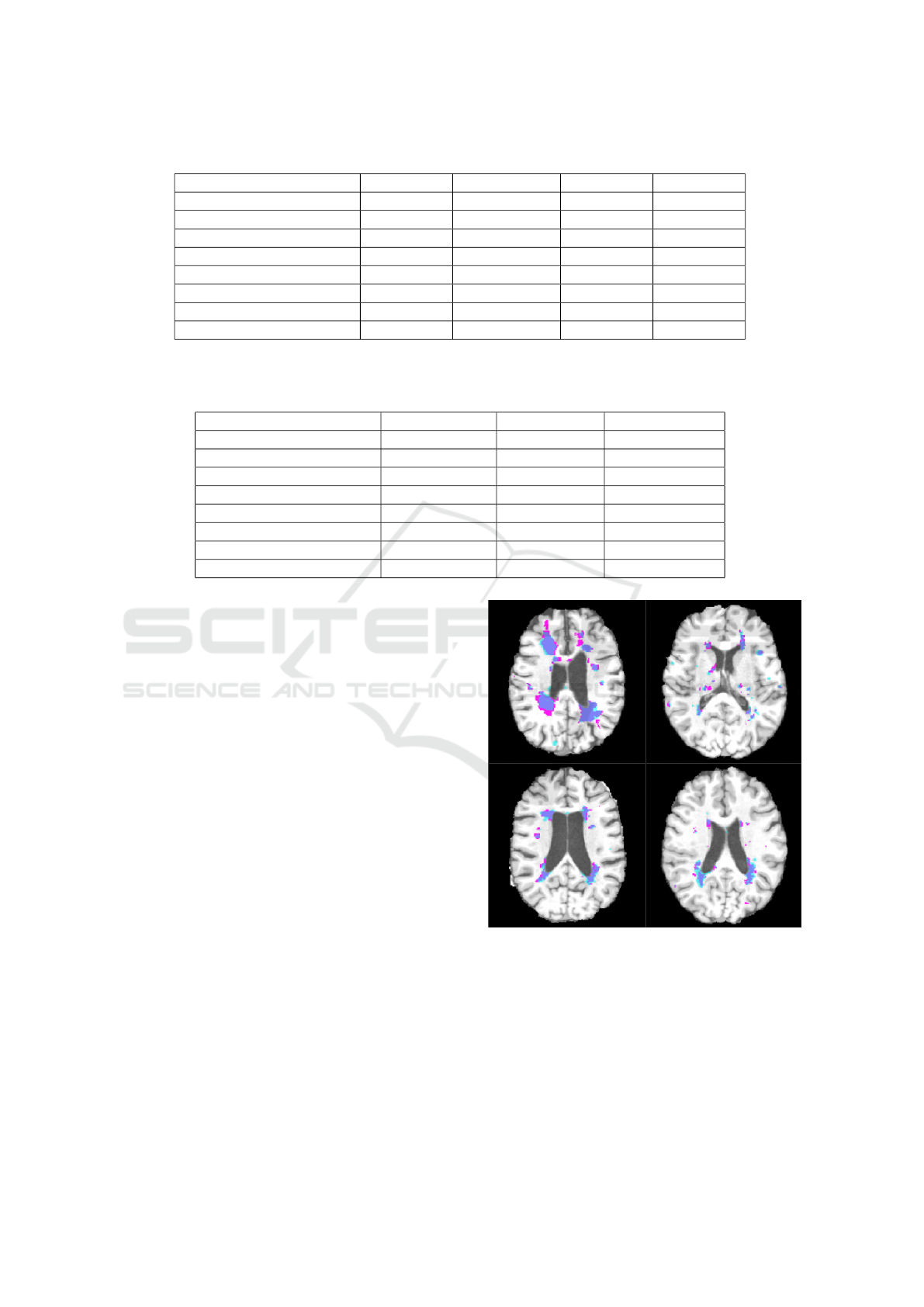
Table 1: Final comparison between models based on DSC, VD, TPR and FDR.

METHOD DSC% VD% TPR% FDR%

LST (LST, 2017) 42.0 ± 19.6 76.7 ± 98.0 49.0 ± 18.3 59.6 ± 22.1

Patch11- w/o location 32.8 ± 21.1 746.5 ± 891.2 81.8 ± 6.6 77.2 ± 16.9

Patch 11- with location 32.7 ± 18.7 650.3 ± 721.1 86.0 ± 9.1 78.2 ± 14.0

Patch 19- with location 45.2 ± 20.1 160.5 ± 212.3 62.5 ± 16.8 60.8 ± 20.3

Patch 11- Cascade 45.3 ± 16.0 178.6 ± 145.7 76.4 ± 14.1 66.2 ± 14.5

Patch 11- 4 class 37.3 ± 16.9 333.9 ± 285.5 79.8 ± 10.3 74.3 ± 13.7

Patch 11 - 3 class 54.8 ± 13.9 39.6 ± 33.8 61.4 ± 14.5 48.2 ± 16.2

Patch 11 - 3 class, Cascade 57.5 ± 12.4 22.8 ± 16.5 59.7 ± 14.6 42.5 ± 14.3

Table 2: Final comparison between models based on # Lesion Voxels found (#LV found), # Lesion CC found (#LCC found)

and # Lesion CC which coincide in GT and found (#LCC coincide). Note that # Lesion Voxels in GT is 11573 ± 9873 and #

Lesion CC in GT is 125.6 ± 61.4.

METHOD #LV found #LCC found #LCC coincided

LST (LST, 2017) 12936 ± 10231 25.3 ± 9.4 31.8 ± 16.6

Patch11- w/o location 36848 ± 11170 561.3 ± 128.6 92.3 ± 41.6

Patch 11- with location 38765 ± 18541 474.9 ± 90.3 91.9 ± 42.2

Patch 19- with location 17468 ± 13073 151.7 ± 62.6 51.6 ± 29.5

Patch 11- Cascade 24695 ± 19621 113.8 ± 38.8 69.9 ± 37.0

Patch 11- 4 class 30826 ± 20973 257.1 ± 42.7 85.1 ± 37.6

Patch 11 - 3 class 13190 ± 11721 150.1 ± 51.8 75.2 ± 38.0

Patch 11 - 3 class, Cascade 11981 ± 10986 101.7 ± 50.4 72.7 ± 31.5

that was contrary to the MS lesion deﬁnition, which

caused some ”wrong” FN in our results and this might

be explained with some special case, a human error or

an error in the alignment process of the images. More

detailed qualitative results can be seen from Figure 6.

From our observations, the model seems to cap-

ture the hypo-intensity in T1 and hyper-intensity in

T2 technically but misses some of the intuitions, dom-

ain knowledge or the subjectivity of the human ex-

pert. The lesions are detected by the proposed mo-

del in hypo-intense regions in T1 and hyper-intense

regions in T2 and the borders are determined by T1

hypo-intense region, which is the correct behavior.

Another positive property of the automatic seg-

mentation is that in the majority of the lesions there

is some detection on the lesion or very close to the

lesion, although the overlapping is far from perfect.

For instance, if seen from a cross-section, there is a

GT lesion that seems not detected, when we advan-

ced a few voxels up or down along the perpendicular

axis of the cross-section, we observe, in most cases, a

lesion detected by the model. This could be due to the

difﬁculty in determining the real borders of a lesion.

In Figure 5 we can see that the number of auto-

matically detected lesion voxels increased with the

number of GT lesion voxels. This means that the seg-

mentation result of our model is indicative of the real

lesion load. This information can be used to see the

progression of the lesions in an MS patient.

Figure 3: Segmentation result, with the best model, of four

subjects in axial plane. TP: Dark Blue, FP: Light Blue, FN:

Pink. Better visualization in pdf.

In terms of computational cost, we observe that

changing the patch size from 11x11x11 to 19x19x19

increases the computational time to more than twice

its original value (approximately, 6 hours as oppo-

sed to 14 hours in the AWS conﬁguration (Amazon,

2017) we chose), but proportionally less than the in-

crease in the number of initial features, which is:

VISAPP 2018 - International Conference on Computer Vision Theory and Applications

266

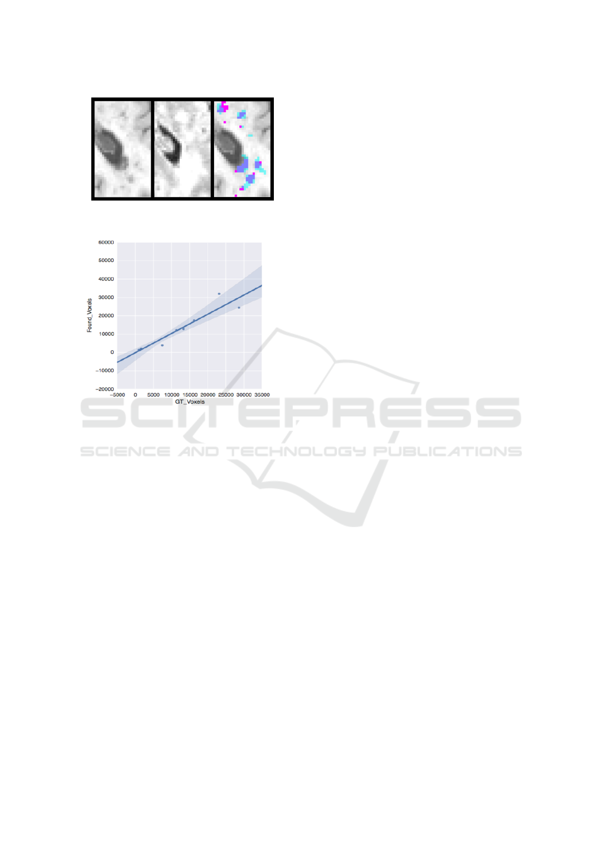
Figure 4: From left to right: T1, T2 and Segmentation re-

sult, close-up from a lesion region. Better visualize in pdf.

Figure 5: The number of Ground Truth lesions vs. the num-

ber of lesions found.

(19/11)

≈ 5.2. The application of the cascade, on

the other hand, increases the computational time ap-

proximately to twice its original value, which is ex-

pected since we train the same size CNN with the

same number of samples twice (additionally the time

for evaluating the training set with the ﬁrst model,

which is negligible in comparison). Increasing the

class size, however, has less dramatic effect on the

computational time causing comparatively a smaller

increase than twofold.

4 CONCLUSIONS AND FUTURE

WORK

In this paper, we have studied several CNN models for

the MS lesion segmentation problem. We have started

with model deﬁnitions from similar approaches in the

literature and we have developed our ﬁnal proposal

by adding new design decisions: deﬁning a new sub-

sampling process, including lesion location informa-

tion in the CNN input, considering a 3-classes classi-

ﬁcation problem and adding a two-stage cascade. We

have shown that these improvements have a positive

effect on the ﬁnal performance. We have shown that

using DL with an appropriate design, we can deﬁne a

method that learns the general rule for MS lesion seg-

mentation. We have obtained promising results for

all the validation measures on a real dataset of 59 pa-

tients from Hospital Cl

ınic. Moreover, the results re-

present signiﬁcant improvement over the commonly

used automatic method of LST. The proposed mo-

del have been able to detect the lesion regions, which

have different intensity values in MRI with respect to

their neighborhood, meaning that it has captured the

mathematical relationship between a 3D patch and the

class of its center voxel to a certain degree. Although

it has captured the general relationship, it has failed to

learn some exceptions requiring domain knowledge

that are applied by human experts during MS lesion

segmentation. This limitation could be due to the fact

that there is not enough cases in the training set for

such exceptions or that it is necessary to feed more

information to the CNN (e.g. more context) for the

model to capture these patterns.

As future work we plan to add more information

about the context and brain spatial dependencies in

order to improve the results. Although we have ad-

ded the location information to add some context, this

may not have been enough since the training set may

not be representative of the exceptions. Thus, adding

the resulting lesion/non-lesion label information (de-

tected by the model) of the neighboring voxels in the

evaluation of a voxel may help achieve better classiﬁ-

cation. In order to include these spatial dependencies,

we can consider Conditional Random Fields as a se-

cond stage.

In the literature, Restricted Boltzmann Machines

(RBM) or auto-encoders have been used to obtain an

initial representation of the data, which could lead to

better classiﬁers. This type of unsupervised methods

can also take advantage of unlabeled data. Therefore,

it might be a good idea to start with an RBM or auto-

encoder and apply our models subsequently.

Finally, another improvement may come from in-

creasing the number of MRI modalities during trai-

ning. We used T1, T2 but adding more modalities

such as FLAIR, fMRI, diffusion MRI could give more

information about the nature of a voxel.

ACKNOWLEDGEMENTS

This work was partly supported by the Ministry of

Economy, Industry and Competitiveness of Spain

(TIN2015-66951-C2-1-R and TIN2013-47008-R), by

Catalan Government (2014-SGR-1219 and SGR-

1187), the EU H2020 and a NVIDIA GPU Grant.

Multiple Sclerosis Lesion Segmentation using Improved Convolutional Neural Networks

267

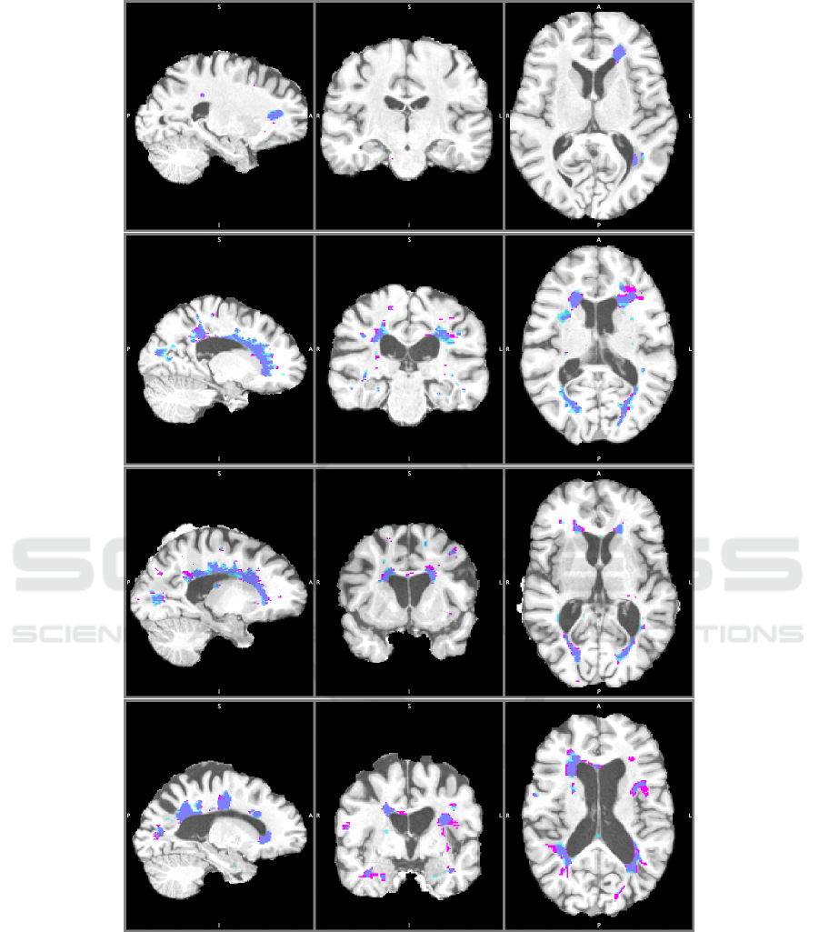
Figure 6: Other segmentation results, with the best model, of four subjects in saggital, coronal and axial plane. TP: Dark

Blue, FP: Light Blue, FN: Pink. Better visualization in pdf.

REFERENCES

Havaei, M., Guizard, N., Larochelle, H. and Jodoin, P-M.

(2016). Deep learning trends for focal brain pathology

segmentation in MRI. arXiv:1607.05258

Greenspan, H., Van Ginneken, B. and Summers,R. M.

(2016). Deep Learning in Medical Imaging: Over-

view and Future Promise of an Exciting New Techni-

que. IEEE Transactions on Medical Imaging, 35 (5),

pp. 1153-1159, 2016.

Garcia-Lorenzo, D., Francis, S., Narayanan, S., Arnold, D.

L., Collins, D. L. (2013). Review of automatic seg-

VISAPP 2018 - International Conference on Computer Vision Theory and Applications

268

mentation methods of multiple sclerosis white matter

lesions on conventional magnetic resonance imaging.

Medical Image Analysis, 17 (1), pp. 1-18, 2013.

Vaidya, S., Chunduru, A., Muthu Ganapathy, R., Krish-

namurthi, G. (201). Longitudinal Multiple Sclerosis

Lesion Segmentation Using 3D Convolutional Neural

Networks. IEEE International Symposium on Biome-

dical Imaging, New York, April 2015.

Brosch, T., Yoo, Y., Tang, L.Y., Li, D.K., Traboulsee, A.,

Tam, R. (2015). Deep convolutional encoder networks

for multiple sclerosis lesion segmentation. Medical

Image Computing and Computer-Assisted Interven-

tion (MICCAI) 2015, pp. 3-11. Springer.

Brosch, T., Tang, L., Yoo, Y., Li, D., Traboulsee, A. (2016).

Deep 3d convolutional encoder networks with short-

cuts for multiscale feature integration applied to mul-

tiple sclerosis lesion segmentation. IEEE Transactions

on Medical Imaging, 35 (5), pp. 1229-1239, 2016.

Ghafoorian, M., Karssemeijer, N., et al. (2017). Location

sensitive deep convolutional neural networks for seg-

mentation of white matter hyperintensities. Scientiﬁc

Reports 7 (1): 5110, 2017.

Valverde, S., Cabezas, M., et al. (2017). Improving auto-

mated multiple sclerosis lesion segmentation with a

cascaded 3D convolutional neural network approach.

NeuroImage, 155, pp. 159-168, 2017.

Plis, S. M., Hjelm, D. R., Salakhutdinov, R., Allen, E. A.,

Bockholt, H. J., Long, J. D., Johnson, H. J., Paulsen, J.

S., Turner, J. A. and Calhoun, V. D. (2014). Deep le-

arning for neuroimaging: a validation study. Frontiers

in Neuroscience, 8, 2014

Goodfellow, I., Bengio, Y., Courville, A. (2016). Deep le-

arning. MIT Press Book.

Bengio, Y. (2012). Practical recommendations for gradient-

based training of deep architectures Neural Networks:

Tricks of the Trade, pp. 437-478, 2012.

National MS Society. http://www.nationalmssociety.org/

Deep Learning. http://deeplearning4j.org/

Freesurfer for processing and analyzing brain MRI images.

https://surfer.nmr.mgh.harvard.edu/

MS Lesion Segmentation Tool (LST). http://

www.statistical-modelling.de/lst.html

Neuroimaging in Python (Nibabel). http://nipy.org/nibabel/

Scikit-learn pre-processing package. http://scikit-learn.org/

stable/modules/preprocessing.html

Amazon Web Services. https://aws.amazon.com/

Multiple Sclerosis Lesion Segmentation using Improved Convolutional Neural Networks

269