Speeding up the Search of a Global Dynamic Equilibrium

from a Local Cooperative Decision

ebastien Maignan, Carole Bernon and Pierre Glize

IRIT, Universit

e de Toulouse, Toulouse, France

Keywords:

Multi-Agent System, Adaptation, Cooperation, Dynamic Equilibrium.

Abstract:

Systems composed of many interdependent active entities working on shared resources can be challenging to

regulate and multi-agent simulation is an efﬁcient means for ﬁnding the suitable entities’ behaviors. On the

other hand, the search space for a stable solution of the system is usually forbidding and hinders any effort

to solve the problem using a top-down approach. Furthermore, the complexity of possible global functions

to optimize increases rapidly with the size of the system and can prove difﬁcult to deﬁne and/or evaluate at

each system simulation step. The difﬁculty when designing bottom-up systems is to be able to identify all

their emergent properties and the parameters to modulate them. Here we propose a local cooperative decision

making process that helps to stabilize such systems. These local processes prove to be very efﬁcient to quickly

ﬁnd dynamic equilibrium solutions where the system continues to function and fulﬁlls its global function.

Regulation emerges from simple local interactions.

1 INTRODUCTION

As opposed to a stable equilibrium, a dynamic equi-

librium is a balanced state which requires negative or

positive feedbacks to stay in its steady state.

In order to remain functional or to operate in an

efﬁcient manner, complex dynamical or open sys-

tems often need to reach such a dynamic equilibrium.

Economy (Aruoba et al., 2006), ﬁnance (Shimomura,

1998), ecology (Tuljapurkar and Semura, 1977) or bi-

ology (Bernado and Blackledge, 2010) are a few ex-

amples of areas in which such systems may exist.

As such, this study focuses on how a dynamic

equilibrium may take place in cellular complex sys-

tems by modelling early stages of cell communi-

ties where interdependent cell species live together,

but without having developed a communication sys-

tem. Theoretically, a dynamic equilibrium should be

reached for every cell to continue to exist and share

resources. In principle, achieving such a state is pos-

sible if actions performed by the system’s cells are

speciﬁcally suited to give the feedbacks required.

A complex system is subject to unexpected behav-

iors due to bifurcations, non linearities, openness; and

consequently cannot be designed in a top-down ap-

proach. A bottom-up design, where the global func-

tion of the system emerges from the interactions of

its more basic components, becomes unavoidable and

makes knowledge of the suited actions impossible.

Finding a way to constrain the actions locally made

by the basic components for speeding up the conver-

gence of the global system toward a dynamic equilib-

rium becomes therefore necessary.

The aim of this paper is thus to study how reach-

ing this dynamic equilibrium can be sped up if local

cooperation is used by the basic components.

Numerous works on cooperation found their ori-

gin on the computer tournament in the 1980s, based

on Robert Axelrod’s “The Evolution of Cooperation”

(Axelrod, 1984). Usually the payoffs in game theory

are ﬁxed, which cannot be the case in the general sit-

uations such as the ones presented in this paper. The

kind of cooperation we consider is seen as helping the

most critical component in the system (Georg

e et al.,

2011), it is not simple cooperation towards a common

goal (Hogg and Huberman, 1992) nor pure altruism;

it is rather seen as benevolence.

For this study, multi-agent based simulation is

used as it is known to be an efﬁcient approach to

simulate complex systems and study their properties

(Moss, 2000). We consider a system where inter-

dependent cells of different types are indirectly ex-

changing resources via a common environment. Ex-

changes are made using basic actions: a cell is able

to gather resources from the environment, to inter-

nally transform some resources into others, and to

Maignan, S., Bernon, C. and Glize, P.

Speeding up the Search of a Global Dynamic Equilibrium from a Local Cooperative Decision.

DOI: 10.5220/0006540101430150

In Proceedings of the 10th International Conference on Agents and Artiﬁcial Intelligence (ICAART 2018) - Volume 1, pages 143-150

ISBN: 978-989-758-275-2

143

release resources in the environment. The studied

system is simulated as a Multi-Agent System (MAS)

(Wooldridge, 2009) where cells are agents situated on

nodes of a grid that form their environment. These

cells are not aware of their neighbors’ actions, are

not able to directly communicate with them, and are

only able to act for gathering, producing or transform-

ing resources units. A cell-agent may live a certain

amount of time depending on the current resources it

possesses and should it die, its node is in charge of

ﬁnding a replacement. Once released by a cell-agent

at a particular node of the environment, a resource

may circulate and be gathered by another cell-agent

on its own node. The environment also produces re-

sources and regenerates the cells when they disap-

pear; and, in this sense, nodes are also considered as

agents because they take decisions for processing this

regeneration.

The aim is therefore to endow agents with purely

local behaviors based on cooperation in order to

study how the simulated system behaves globally and

whether these cooperative behaviors enable ﬁnding a

dynamic equilibrium in an efﬁcient manner. In other

terms, we want to verify whether cooperation, as de-

ﬁned here, is an effective behavior to build an agent-

based simulation in a bottom-up way considering that

agents, as in real life, have a very limited knowledge

of their surrounding and no knowledge at all of the

global state to reach.

The paper is structured as follows. The features of

the studied system as well as the cooperation used for

replacing component-agents and selecting their ac-

tions are presented in section 2. Section 3 presents

some results when cooperation is used in systems

with populations of 2 or 10 component species. Be-

fore concluding in section 5, section 4 studies the sta-

bility and robustness of the cooperative heuristics.

2 SIMULATED SYSTEM

As mentioned earlier, the studied system simulates

early stages of cell communities where interdepen-

dences exist between cell types but no communication

system exists yet to coordinate their actions. While

being a very simpliﬁed version of actual cell commu-

nities, this system is already complex enough to ob-

serve emergence of some interesting behaviors.

Cells are the interdependent components of the

system, they release into or gather, from the environ-

ment, molecules representing resources which they,

as a whole, require to survive. Reaching a dynamic

equilibrium in such a cellular system means that all

the cells ﬁnd a way to survive by exchanging the right

resources in the right way without having any prior

knowledge about this. The system template is loosely

based on cell communities sustaining each other by

producing speciﬁc resources required by other cell

types and receiving vital resources from other mem-

bers of the community. The working model of each

cell is a very simpliﬁed version of actual cells and

only gathering, release and production functions have

been kept.

This section presents the general features of the

simulated system and describes the cooperative be-

haviors used by its agents in order to reach a dynamic

equilibrium in a faster way. The parameters actually

used for the simulation are given in section 3.

2.1 System

The simulated system has therefore two parts: cell

agents (later on, simply “cells”) and their environ-

ment. This environment is a two-dimensional tore

seen as a grid of node agents (later on, simply

“nodes”) on which cells are regularly placed.

A given number of resources (nR) are available in

the system. Each node of the environment contains

external resources eR

where i is the resource index.

Each cell contains internal resources iR

and a set of

actions. Three different types of actions enable a cell

to act on resources:

• Gathering: Transfers a given amount from the

node resource eR

to the cell resource iR

• Production: Transforms a given amount of lin-

ear combination of iR

s into another kind iR

i.e.

∑

.iR

→ iR

where

∑

= 1.

• Release: Transfers a given amount of cell resource

to the node resource eR

Only one action can be performed by a cell dur-

ing each simulation cycle. Performing this action will

cost the cell a certain amount of one particular re-

source that can be viewed as its energy source. How-

ever, as in real life, a cell does not have any knowl-

edge that a particular resource is actually its energy

source and is therefore unable to optimize its behav-

ior towards energy maximization.

The longer a real cell exists the more errors it

will accumulate. These errors are simulated by giving

each cell a probability to disappear which increases

with its age. When a cell fails, it is immediately re-

placed on the node it occupied (see section 2.4).

Internal or external resources are divided into two

subsets: SetA = {R

, i ≤

}, which contains abun-

dant resources supplied by the nodes, and SetB =

, i >

}, which contains resources only produced

ICAART 2018 - 10th International Conference on Agents and Artiﬁcial Intelligence

144

by cells. Resources from SetA are replenished ev-

ery cycle either at each node and are always available

to cells. On the contrary, a constant amount of re-

sources from SetB is removed every cycle from ev-

ery node to simulate their transport away from the

system. Resources diffuse from high content nodes

to low content neighboring nodes

. To summarize,

there are three mechanisms to modify resource con-

tent at each nodes: passive diffusion, active gath-

ering/release from cells and outside world inﬂuence

(positive for SetA and negative for SetB).

The overall goal of the system is to reach a dy-

namic equilibrium and to provide a steady output

of resources from SetB. Robustness to resources

changes and/or component distribution is also an im-

portant criterion to consider.

As introduced before, cooperation is used to reg-

ulate the actions performed by the cell/node agents in

the system, and it is supposed that every agent knows

that its neighbors expect reciprocal cooperation. A

cooperative behavior is a balance between selﬁshness

and altruism and is implemented in two parts: (1) dur-

ing the action selection for each cell (see section 2.3),

and (2) during the creation of a new cell (see section

2.4).

2.2 Resources Criticality

The notion of criticality is used by a cooperative agent

to decide which agent is considered as having the

highest degree of dissatisfaction in its neighborhood

(No

el and Zambonelli, 2015) in order to help it if pos-

sible.

Here, cells do not know how other cells perform

so their degree of dissatisfaction can only be related

to resources variations. Thus internal and external re-

sources criticalities reﬂect this information. In the

same way, nodes also require access to external re-

source criticality to operate the cooperative agent re-

placement process (see section 2.4).

Resource criticality is a measure of the current

available quantity of a resource combined with its

forecast availability. The current available quantity

of a resource could translate as “is it rare or plenti-

ful?”. Its forecast availability could translate as “is it

disappearing from the environment or not, and how

fast?”. So, an abundant resource replenished every

cycle will have a very low criticality whereas a very

rare resource consumed by all neighbor cells will have

a very high criticality. Whatever the actual numerical

The fact that cells are immobile does not reduce the

problem scope since resources may move and each agents

neighborhood changes over time.

implementation of the criticality evaluation, its fun-

damental characteristic is that it can be compared and

ranked.

Criticality is a local measure available only to a

single cell and its containing node.

2.3 Cooperative Action Selection

Process

Every cycle, each cell selects an action and performs

it.

The default algorithm, for comparison purposes,

consists in randomly choosing this action. The ac-

tion selection process proposed is based on coopera-

tion between cells to improve the status of resources

in critical situations.

Firstly, resources criticalities for all resources, in-

ternal and external, are calculated and ranked.

All actions that could be performed by the cell are

then put in a working set. For example, a gathering

action will only be added if the external resource this

action involves is available in the environment.

Starting from the most critical resource, actions

from the working set are sorted according to their pos-

itive impact on this resource i.e. the amount of re-

source it would add either internally or externally. If

several actions have the same impact, the one with the

least impact on other resources is selected. If no ac-

tion can improve the status of this critical resource,

the next most critical resource is evaluated. If no ac-

tion can improve the status of any critical resource, a

random action is selected.

The ﬁnal action selected after this process is then

performed by the cell.

This process will select all the necessary actions to

gather, produce and release all the resources ensuring

the cell’s survival and that of its neighbourhood.

Several experiments (data are not shown here)

proved that a random selection of actions always

quickly leads to a global system failure. In conse-

quence, all the results presented thereafter use the co-

operative process for action selection.

2.4 Cooperative Agent Replacement

Process

Any given cell can fail for two reasons: it has become

too old or its energy resource has fallen to zero. A

failed cell disappears and needs to be replaced so that

each node of the system is occupied at all time. The

new cell has to be the daughter of an existing cell from

its neighbourhood.

All cells in a speciﬁc radius (small compared to

the system size) around the failed cell position are

Speeding up the Search of a Global Dynamic Equilibrium from a Local Cooperative Decision

145

candidates to replace it, but only those with enough

energy resource to last a predeﬁned number of cycles

are considered as potential candidates.

The default algorithm, applied by a node to re-

place the cell which failed at its location, consists of

randomly selecting one of the potential candidates.

The agent replacement process proposed uses coop-

eration to make the node select the candidate that will

help the most critical external resource in its direct

neighborhood.

Only external resources are used during this pro-

cess since the nodes and cells do not have any knowl-

edge of the resource content in the neighboring cells.

A node has access to resource criticalities (as deﬁned

in section 2.2) in the neighboring nodes. This is the

way to make cooperation possible.

First, for each resource eR

, its criticalities on each

neighboring nodes are calculated and compared, and

the worst one becomes the criticality for eR

Then, starting from the most critical eR

, candi-

date cells are ranked according to the amount of iR

they released in the recent past. If more than one can-

didate released iR

, they are ranked by the amount

released and the top half remain candidates for the

next comparison round using the next most critical

resource. This is repeated until only one candidate

remains or all critical resources have been tested. The

right candidate is then duplicated (i.e. with its current

sets of resources and actions) to the failed cell posi-

tion.

If there are no candidates, the node stays empty

and the process starts over during the next cycle. This

can potentially lead to full system halt if mass cell

failure occurs.

3 SIMULATION RESULTS

In order to evaluate the efﬁciency of local cooperation

– as described in the previous section – to regulate a

running system, several simulations were performed

and are described in this section. After describing

how the simulation is initialized, results are given for

simulations where 2 or 10 interdependent cell types

are considered.

3.1 System Initialization

“Abundant” resources from SetA are distributed ran-

domly on the nodes of the system and within the

cells. “Rare” resources from SetB are distributed ran-

domly within the cells to provide them with enough

energy resources to survive for at least a given num-

ber (nMinS) of cycles.

Initially, nCa cell types are distributed on the sys-

tem nodes; these types are classes of cells that differ

by their energy resources and their production action.

For each cell type j ∈ {1, ..., nCa}, one resource

from SetB is chosen as the energy source for this type

(which is not known by the cells). Furthermore, this

cell type is given a set of actions: shared common

actions to gather or release any type of resource, along

with one speciﬁc production action allowing this cell

type to produce one unit of its energy resource using

units of one resource from SetA and a

units of

one resource from SetB:

.iR

+ a

.iR

( j+1+

) mod nCa

→ iR

( j+

)

with

+ a

= 1

At the start of the simulation, each cell instance of

a given type j has a unique random set of (a

, a

To illustrate this a 2-cell type and 4-resource sys-

tem would give the following cyclic interdependence:

cell type 1: a

.iR

+ a

.iR

→ iR

cell type 2: a

.iR

+ a

.iR

→ iR

In other words, each cell is able to produce its en-

ergy resource but needs resources only produced by

another cell type to do so. Without any knowledge

about its energy resource, and although it is vital to

its survival, a cell must somehow manage to release

some of it so that other cell types can survive.

The proportion and location of cells using a spe-

ciﬁc energy resource can be set randomly or following

a predeﬁned pattern. In all the following examples,

cells of a given type are spatially grouped together at

the beginning of the simulation and the proportions

for each cell type are the same.

For the results given hereinafter, the features of

the simulated system are as follows: nCa is set to 2 or

10, nR is set to 20 i.e. SetA = {R

...R

} and SetB =

...R

} and nMinS is arbitrarily set to 80.

The size of the simulated system is 60 × 60 with

3600

nCa

of the cells for each type. The speed at which

resources can move from one node to its neighbors

(diffusion factor) is set to 0.01 unit/cycle. The radius

for candidate selection is set to 4 nodes in the coop-

erative agent replacement process: this is larger than

the direct neighborhood of a node using a radius of 1

(involving 8 nodes) but lower enough for not consid-

ering the whole grid as its neighborhood.

A rough estimation of the parameter space for the

system is as follows: every cycle, each of the 3600

cells may perform 1 out of 40 actions that are common

to all cell types, and 1 action, speciﬁc to its type. Con-

sidering that cell type populations are roughly equiv-

alent, there are (40 + nCa)

3600

possible choices every

cycle. As observed in several simulations, the system

can be balanced within 1000 cycles.

ICAART 2018 - 10th International Conference on Agents and Artiﬁcial Intelligence

146

The parameter space for this period is therefore at

least (40+nCa)

3600

1000

. Random walk in such a huge

space is very unlikely to succeed. Actually, starting

from an identical initial state, in all the experiments

performed none of the system conﬁgurations of the

random simulation ever matched one of the coopera-

tive simulation.

We are fully aware that comparing the results ob-

tained by the system, when cooperation is used to

constrain the actions performed locally by the agents,

with other works in the same vein is compelling.

However, to the best of our knowledge, we did not

ﬁnd simulations of similar systems to perform such a

comparison. Furthermore, since a global cost func-

tion cannot be considered to use machine learning ap-

proaches such as neural networks (Colak, 2006) or

genetic algorithms (Gen and Cheng, 2000), we chose

to randomly explore the search space to show the dif-

ﬁculty to ﬁnd solutions and their sparsity.

3.2 Two Interdependent Cell Types

For this scenario, there are nCa = 2 cell types.

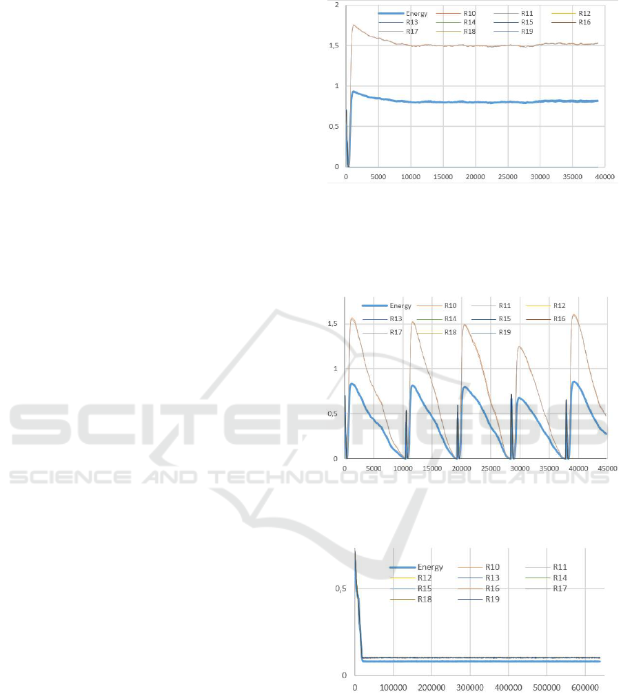
The cooperative system quickly reaches a dy-

namic equilibrium (ﬁgure 1) whereas random selec-

tion of new cells cannot maintain a dynamic equilib-

rium after the stabilization period (ﬁgure 2).

In ﬁgure 1, resources R

to R

quickly disappear

from the system since none of the two cell types can

produce or use them. These resources are then always

the most critical ones but no action can improve their

state. This is not a problem for the system as a whole

as these resources do not impact the viability of the

cells.

It is noteworthy to mention that the spatial distri-

bution of type 1 and type 2 cells is not regular and

does not display any kind of (visually) distinctive pat-

tern (result not shown here).

Interestingly after a few thousand cycles, only one

instance of type 1 and one instance of type 2 cells are

left from the initial random sets and occupy all the

simulation space. It can be noted that the surviving

instances selected by the cooperation process always

have a

above 0.8 and a

below 0.2. This can be

explained by the fact that cells using more scarce re-

sources from SetB will have a shorter lifespan and be

replaced more often. This indicates that the system

maximizes the use of abundant resources (R

to R

)

and minimizes the consumption of rare resources (R

and R

3.3 Ten Interdependent Cell Types

For this scenario, there are nCa = 10 cell types.

Figure 1: Result of dynamic equilibrium between 2 interde-

pendent cell types using cooperation. The x axis represents

the number of simulation cycles. The mean quantity of each

resource from SetB(R

−R

) in the nodes (top curve) and

the mean energy of the cells (bottom thicker curve) are rep-

resented on the y axis. R

and R

are nearly superimposed

and R

−R

are equal to zero very early in the simulation.

Figure 2: Same setup as Fig. 1 but using random selection

for failed cells. Each spike denotes a system restart when

at least one component type disappeared compromising the

future of the whole system.

Figure 3: Result of dynamic equilibrium between 10 in-

terdependent cell types using cooperation. Resources are

nearly surimposed and show very small ﬂuctuations (bot-

tom curve).

As shown in ﬁgure 3, after around twenty thou-

sand cycles the system reaches a dynamic equilibrium

using the cooperation selection process (contrary to

ﬁgure 4 where the random one is used). All resources

from SetB are used by one cell type or another. This

explains why none of the resource quantities falls to

Speeding up the Search of a Global Dynamic Equilibrium from a Local Cooperative Decision

147

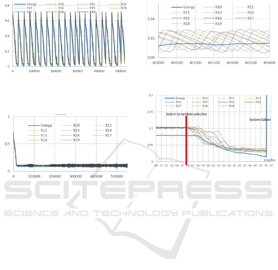
Figure 4: Same setup as ﬁgure 3 but using random selection

for failed cells. The number of cycles before failure may

vary but the system is always unstable and never reaches

a dynamic equilibrium state (noted also in all the different

random simulations launched).

Figure 5: Same setup as ﬁgure 3 but using a slower resource

diffusion factor (10×). This impacts the resource values and

the cell type distribution. The ﬂuctuations are cyclic instead

of random.

zero.

Again, when the system becomes stable, it is ﬁlled

with instances for which a

is above 0.8 and a

below 0.2.

Using the same system setup but with a much

slower diffusion factor (10 times slower) the sys-

tem behaves slightly differently (see ﬁgures 5 and 6).

Fluctuations of a resource R

become cyclic and cor-

related with those of R

j−1

and R

j+1

. This correlation

is the result of resource coupling in the production ac-

tions of the interdependent cell types. The diffusion

factor impact can be explained by the fact that cells

will deplete the medium of resources they need be-

fore they can be replenished by the passive diffusion

mechanism. Cells will start to die but resource quan-

tities will allow a small population to subsist. Even-

tually diffusion will replenish the depleted resources

and cells will thrive again.

In parallel, cell type populations also present

cyclic and correlated behaviors (these data are not

shown). Although in most simulations the system is

dynamically stable, it happened on some occasions

that the ﬂuctuation amplitudes increased with time

and led to system failure.

Figure 6: Same setup as ﬁgure 5 showing the resource oscil-

lations and interdependence. Cell type population displays

a similar oscillating behavior.

Figure 7: When a stabilized system is switched to random

selection of new cells, it oscillates for a while before even-

tually failing after around 15000 cycles (when one cell type

vanishes from the system). For clarity, cycles 0-50000 were

removed.

4 COOPERATION AND

DYNAMIC EQUILIBRIUM

Through three experiments derived from the simula-

tion used in section 3.3, this section studies how ro-

bust is cooperation when a certain percentage of cells

are replaced using the basic random algorithm.

4.1 Solution Stability without

Cooperative Selection

Using the scenario and solution found in section 3.3

with 10 cell types, the system is switched from a co-

operative selection of new cells to a random one.

At the time of the switch, {(a

, a

)} for the pro-

duction actions of all cells has been optimized by the

cooperation for the best possible performance. The

consequence is that the system is able to survive for

much longer than a new system using the much wider

selection of {(a

, a

)} available at the simulation

start. Nevertheless, as illustrated in ﬁgure 7, after

several thousand cycles the equilibrium between cell

types is not maintained and the system fails.

ICAART 2018 - 10th International Conference on Agents and Artiﬁcial Intelligence

148

4.2 Robustness to Noise

This scenario studies the robustness to noise of the

cooperative algorithm described in section 3.3. Each

time a cell needs to be replaced there is a given prob-

ability to use the random selection or the cooperative

process.

An insight of the effect of cooperation is given in

ﬁgure 8. The cooperative process is efﬁcient in sta-

bilizing the system even when new cells are selected

randomly 99% of the time. Nevertheless, at high ran-

dom percentage the system is more sensitive to ini-

tial conditions and cell distribution. Statistical stud-

ies need to be performed in order to evaluate the ex-

act percentage of cooperative replacement process re-

quired to hold the system steady.

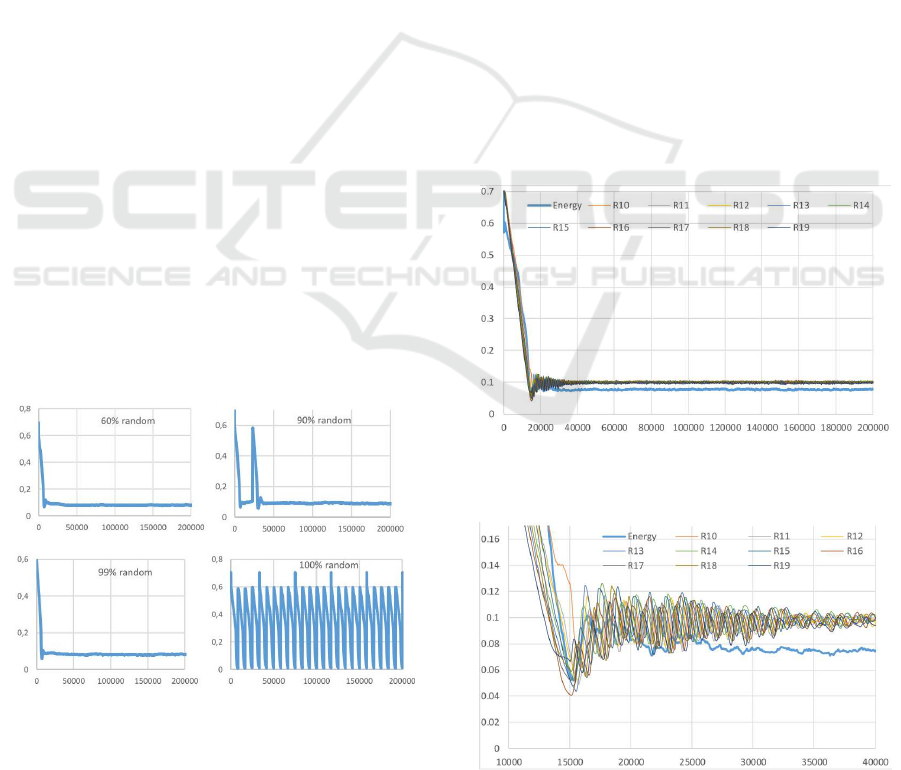
4.3 Saving a Failing System

In this experiment, a system, as described in section

3.3, is simulated using random selection of cells until

failure. Every thousand cycles the system is saved.

Failure occurs after around 23 thousand cycles. Then

every saved instance of the system is continued using

cooperative selection of cells and the system survival

time is measured. This procedure is not equivalent

to restarting the system with different random seeds

since during system restart each cell receives enough

energy resource to survive a given number of cycles.

As shown in ﬁgure 9 and 10, the system can be

saved if cell selection is switched to cooperation early

enough (around 15K cycles). After this time, it is not

possible to rebalance the system. One reason is that

some cell type populations are so low that they can-

not be increased before random failure from old age

Figure 8: These graphs represent the mean cells energy

during the simulation when replacement cells are selected

increasingly randomly. Up to 99% of random selection

the system is still stable. Nevertheless, some of the ran-

dom starting system conﬁgurations cannot be balanced as

demonstrated by the restart pikes observed in most of the

graphs.

or low energy remove them from the system. Another

reason is that the number of instances with interest-

ing {(a

, a

)} for the system balancing might not be

present anymore.

4.4 Scalability

The largest system tested so far consists of a 300×300

grid with 30 cellular types and 60 different resources.

After 5K cycles, the system reaches a dynamic equi-

librium and is still stable after over 62K cycles. Nev-

ertheless due to its size this experiment has not been

repeated extensively and is only mentioned here as an

indicator of the scalability for this approach.

5 DISCUSSION

This article aimed at showing that a speciﬁc kind of

cooperation enables a global dynamic equilibrium to

be found in a faster way than randomly and has used

a multi-agent system to simulate a complex system of

interdependent components where the dynamic equi-

librium means survival of the components.

Figure 9: The system was simulated for 15K cycles us-

ing random selection then switched to cooperative selection.

The system is stabilized and reaches dynamic equilibrium.

Figure 10: Close up on the transition phase from ﬁgure 9

The system oscillates for around 20K cycles before cell type

populations and resources are balanced.

Speeding up the Search of a Global Dynamic Equilibrium from a Local Cooperative Decision

149

Optimizing localized production and consump-

tion of various resources globally can prove to be a

very challenging endeavor. The formal global func-

tion to minimize is not straightforward to derive from

the system description nor to evaluate at each cycle.

Therefore it becomes necessary to endow components

with a local attitude which enables emergence of the

right global behavior. The local actions considered

here always tend to help the most critical entity in the

local environment of the component, as such they are

said to be cooperative.

A cellular system in which resources are produced

or consumed by cells was chosen to perform experi-

ments with a growing number of cell types, and re-

lated results were presented.

As expected from its huge size, a random explo-

ration of the search space is unsuccessful even when

repeatedly tried with different starting systems (these

data are not shown). On the other hand, local cooper-

ation allows components/cells to regulate efﬁciently

the resource management although the global goal of

the system is locally unknown and the cell knowledge

about its neighborhood is quite restricted.

Furthermore, the processing is totally distributed

within the nodes and cells. Their interactions depend

only on a very limited neighborhood: the ones to se-

lect a new cell to duplicate. This makes the simula-

tion very simple to parallelize and reduces computa-

tion time. Also the code of the nodes and cells which

facilitates the progression in the search space is ex-

tremely simple. This stems from the fact that the local

decision based on cooperation replaces the complex-

ity of the global problem.

The result of the resolution process is totally emer-

gent in the sense that no part of the code is guided by

an evaluation of the overall quality of the solution in

progress (which is almost impossible to estimate).

The more resources to regulate the more challeng-

ing the regulation is. In this paper we have demon-

strated that local cooperative processes to select cell

actions to perform and to replace failed components

are able to regulate a system with 10 interdependent

cell types working on 20 resources.

Two interesting observations have been made dur-

ing these simulations. First, the factors in the pro-

duction actions {(a

, a

)} always tend to be large

for abundant resources from SetA and small for scarce

resources from SetB. This is intuitively a good thing

to do when you optimize such a system. Neverthe-

less, this is not coded in the cooperative processes but

emerges from them.

Secondly, the mean value of the resources quan-

tities in the system tends toward a value that is not a

parameter in the system simulation: around 0.8 for 2

cell types, and 0.1 for 10 cell types. These values also

emerge from the cooperative processes and no single

parameter in the simulation seemed to be able to alter

them signiﬁcantly (these data are not shown).

As demonstrated in section 4.1, stabilization of

the system with the cooperative processes must be

continuous since it eventually fails sooner or later if

switched to random selection. Nevertheless, as shown

in section 4.2, only a very small amount of coopera-

tive selection is necessary to continue to stabilize the

system.

REFERENCES

Aruoba, S. B., Fernandez-Villaverde, J., and Rubio-

Ramirez, J. F. (2006). Comparing solution methods

for dynamic equilibrium economies. Journal of Eco-

nomic dynamics and Control, 30(12):2477–2508.

Axelrod, R. (1984). The Evolution of Cooperation. Basic

books.

Bernado, P. and Blackledge, M. (2010). Proteins in dynamic

equilibrium. Nature, 468(7327):1046–1047.

Colak, S. (2006). Neural Networks Based Metaheuris-

tics for Solving Optimization Problems. University of

Florida.

Gen, M. and Cheng, R. (2000). Genetic algorithms and

engineering optimization, volume 7. John Wiley &

Sons.

Georg

e, J.-P., Gleizes, M.-P., and Camps, V. (2011). Co-

operation. In Di Marzo Serugendo, G., Gleizes, M.-

P., and Karageorgos, A., editors, Self-organising Soft-

ware: From Natural to Artiﬁcial Adaptation, pages

193–226. Springer.

Hogg, T. and Huberman, B. A. (1992). Better than the best:

The power of cooperation. SFI, pages 163–184.

Moss, S. (2000). Editorial introduction: Messy systems-

the target for multi agent based simulation. In Multi-

Agent-Based Simulation, pages 1–14. Springer.

el, V. and Zambonelli, F. (2015). Methodological guide-

lines for engineering self-organization and emergence.

In Software Engineering for Collective Autonomic

Systems, pages 355–378. Springer.

Shimomura, K. (1998). A dynamic equilibrium model of

durable goods monopoly. Journal of Economic Be-

havior & Organization, 33(3-4):507–520.

Tuljapurkar, S. and Semura, J. (1977). Dynamic equilib-

rium under periodic perturbations in simple ecosystem

models. Journal of Theoretical Biology, 66(2):327–

343.

Wooldridge, M. (2009). An Introduction to Multiagent Sys-

tems. John Wiley & Sons.

ICAART 2018 - 10th International Conference on Agents and Artiﬁcial Intelligence

150