
Efficient Curvature-optimized G
2
-continuous Path Generation with
Guaranteed Error Bound for 5-axis Machining
Evgenia Selinger
1
and Lars Linsen
1,2
1
Jacobs University, Bremen, Germany
2
Westf
¨
alische Wilhelms-Universit
¨
at M
¨
unster, M
¨
unster, Germany
Keywords:
NURBS Curves, 5-axis Machining, G
2
-continuity.
Abstract:
Automated machining with 5-axis robots require the generation of tool paths in form of positions of the tool
tip and orientations of the tool at each position. Such a tool path can be described in form of two curves, one
for the positional information and one for the orientational information, where the orientation is given by the
vector that points from a point on the orientation curve to the respective point on the position curve. As the
robots need to slow down for sharp turns, i.e., high curvatures in the tool path lead to slow processing, our goal
is to generate tool paths with minimized curvatures and a guaranteed error bound. Starting from an initial tool
path, which is given in form of polygonal representations of the position and orientation curves, we generate
optimized versions of the curves in form of B-spline curves that lie within some error bounds of the input path.
Our approach first computes an optimized version of the position curve within a tolerance band of the input
curve. Based on this first step, the orientation curve needs to be updated to again fit the position curve. Then,
the orientation curve is optimized using a similar approach as for the position curve, but the error bounds are
given in form of tolerance frustums that define the tolerance in lead and tilt. For an efficient optimization
procedure, our approach analyzes the input path and splits it into small (partially overlapping) groups before
optimizing the position curve. The groups are categorized according to their geometric complexity and handled
accordingly using two different optimization procedures. The simpler, but faster algorithm uses a local spline
approximation, while the slower, but better algorithm uses a local sleeve approach. These algorithms are
adapted to both the position and orientation curve optimization. Subsequently, the groups are combined into a
5-axis tool path in form of two G
2
-continuous B-spline curves over the same knot vector.
1 INTRODUCTION
The sculptured surface machining technology has be-
come a widely used technology in manufacturing en-
gineering, e.g., for shaping metal and other solid ma-
terials. A necessary integral part is the generation
of a milling path. The milling machine cuts along a
given path to obtain the required shape of the work-
piece. For 5-axis milling, the cutter rotates around the
spindle axis, the spindle can move in all three spa-
tial directions, and the workpiece is fixed to a table,
which can also move in two angular directions to al-
low the milling tool to have access to the workpiece
from different orientations. The flexibility of 5-axis
machining allow for manufacturing of more compli-
cated workpieces and for higher quality. However, it
requires the control of the five axes. The first three
axes represent the position of the milling tool in form
of xyz-coordinates, the other two are necessary to rep-
resent the orientation of the table to which the work-
piece is attached, i.e., the angle between the milling
tool and the table (see Fig. 1a).
The tool path for 5-axis machining is given in
form of a position curve of the tool tip and a respec-
tive orientation of the tool for each point on the posi-
tion curve. We assume that the orientation is given in
form of an orientation curve, where the implied orien-
tation is given by the vector that points from a point
on the orientation curve to the respective point on the
position curve. As sudden changes in the tool path
requires the robot to slow down to perform the re-
spective movements, it is desirable to have tool paths
with low curvature on both position and orientation
curve. Our goal is to minimize the overall manu-
facturing time, i.e., to generate a curvature-optimized
tool path for 5-axis machining. Our algorithms take
a given tool path and performs an optimization of po-
sition and orientation within given error bounds. As
Selinger, E. and Linsen, L.
Efficient Curvature-optimized G
2
-continuous Path Generation with Guaranteed Error Bound for 5-axis Machining.
DOI: 10.5220/0006537400590070
In Proceedings of the 13th International Joint Conference on Computer Vision, Imaging and Computer Graphics Theory and Applications (VISIGRAPP 2018) - Volume 1: GRAPP, pages
59-70
ISBN: 978-989-758-287-5
Copyright © 2018 by SCITEPRESS – Science and Technology Publications, Lda. All rights reserved
59
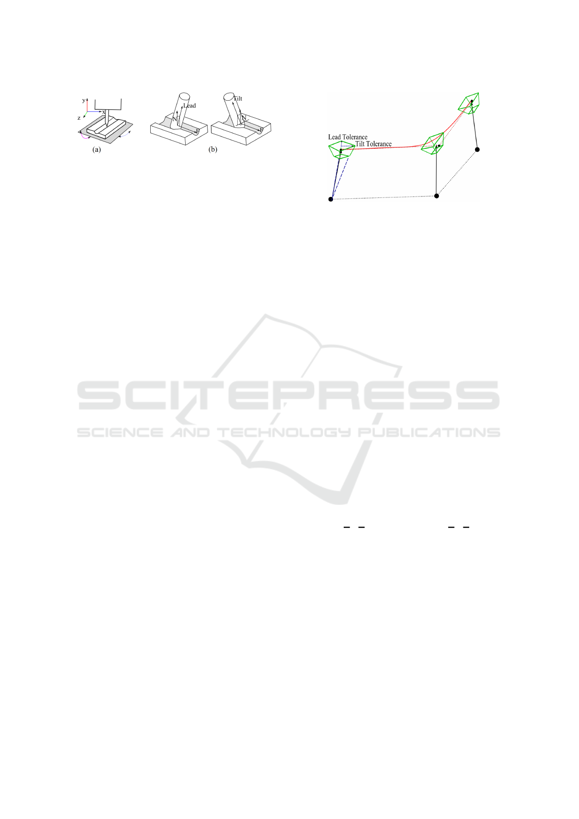
Figure 1: (a) 5-axis machining. (b) Orientational informa-
tion of the tool in form of lead and tilt.
this optimization is embedded into the manufacturing
workflow, it needs to be efficient, as well.
The input to our algorithm is a sequence of pairs
(p,q) of points. The points p are the positions of
the milling tool on the workpiece, the points q are
the orientation points of the milling tool at that time.
When connecting the sequences of points p and q, re-
spectively, they describe the position and orientation
curves in polygonal representation. The orientation
vector q − p given as the difference of the position
and the orientation point can be directed at various an-
gles to the workpiece depending on the desired man-
ufacturing process. The angle is defined by values of
lead and tilt. Lead is the angle between the normal
vector N of the workpiece’s surface and the orienta-
tion vector q − p of the milling tool in the direction
of movement F. Tilt is the angle between the nor-
mal vector N and the orientation vector q − p of the
milling tool perpendicular to the direction of move-
ment F (see Fig. 1b).
Our optimization procedure starts with the opti-
mization of the position curve. The curvature of the
curve shall be minimized within a given tolerance
band. This part of our approach is equivalent to the
optimization for 3-axis machining (Selinger and Lin-
sen, 2011). Then, we need to synchronize the repre-
sentation of the orientation curve with the new (op-
timized) representation of the position curve. Subse-
quently, we perform the optimization of the orienta-
tion curve. To get a desired result we use the restric-
tion that corresponding position and orientation con-
trol points have to form an orientation vector in the
same direction and length as neighboring initial vec-
tors with some small given allowed deviation of lead
and tilt (see Fig. 2). For the synchronization of the
orientation curve with the optimized position curve,
we need to build new orientation vectors starting at
the control points of the optimized position curve with
the direction depending on the direction of the given
neighboring orientation vectors with weights propor-
tional to the distance to them. Based on the given tol-
erances of lead and tilt, we built frustums around gen-
erated orientation points and restrict them lie within
these frustums.
As the optimization of the tool path is embedded
in the manufacturing process, it shall be efficient. We
Figure 2: Black vectors are newly generated orientation
vectors starting from the optimized position control points.
Frustums (green) are built with respect to given tolerances
for lead and tilt (blue). Red curve is the resulting B-spline
orientation curve with the control polygon shown as dotted
dark-red lines.
propose a method that is based on local optimizations,
which are faster to compute than global computations.
Therefore, we first split the toolpath into groups, han-
dle groups individually, and combine the results. The
handling of the individual groups is based on how
complicated their geometry is. Simple groups can be
handled with a simple spline approximation with suf-
ficient quality. Complicated groups are handled using
a more complex sleeve algorithm. Section 3 describes
the overall processing pipeline, which outlines the re-
mainder of the paper.
The resulting position curve is a B-spline curve
C(u) :=
n
∑
j=0
P
j
N
d
j
(u), a ≤ u ≤ b (1)
where the interval [a,b] can be any, P
j
denotes the j-th
position control points, and N
d
j
denotes the j-th nor-
malized B-spline function of degree d. The B-spline
basis functions are defined over a nonperiodic knot
vector
U = (a,··· , a
| {z }
d+1
,u
d+1
,··· , u
m−d−1
,b,··· , b
| {z }
d+1
), (2)
where m = n + d + 1.
The resulting orientation curve shall also be rep-
resented as a B-Spline curve
B(u) :=
n
∑
j=0
Q
j
N
d
j
(u), a ≤ u ≤ b
where Q
j
denotes the j-th orientation control point.
The B-spline basis functions N
d
j
and knot vector U
are identical to the position basis functions and knot
vector.
The B-spline curve constructions assure that the
curves are G
2
-continuous, which is a desired require-
ment for smooth tool paths for machining.
GRAPP 2018 - International Conference on Computer Graphics Theory and Applications
60

2 RELATED WORK
A lot of work has been done in 5-axis milling and one
of the main topics in this context is to find a proper
position and orientation of the milling tool (Jun et al.,
2003). To make the best use of 5-axis machines they
have to solve complicated interference problems and
to determine the optimal tool orientations for com-
plex data machining. Gouging and tool collision (see
Fig. 3) are the main problems in 5-axis machining of
sculptured surfaces. Gouging denotes the removal of
the excess material in the area of the cutter contact
point due to the mismatch in curvatures between the
tool tip and part of the milling path. Collision is the
interference of the cylindrical part of the tool or tool
holder and the workpiece part. The goal is to calculate
an optimal slope of the milling tool based on a given
workpiece trajectory. We, on the other hand, assume
that a tool path is already given. Our goal is to opti-
mize the tool path respect to curvature within an error
bound of the given tool path. Some of existing papers
(Kim and Sarma, 2002; Lavernhe et al., 2007) are us-
ing kinematic constraints to calculate tool path such
as maximum feedrate and acceleration, and also con-
sider the shape of the tool tip, which are not available
for us on this step.
Figure 3: Gouging (left) and collision (right).
In some papers (Fleisig and Spence, 2001;
Langeron et al., 2004) it was suggested to find posi-
tion P(u) and orientation Q(u) B-spline curves by in-
terpolating of position points P
i
and orientation points
A
i
with the restriction that the two B-spline curves sat-
isfy the criterion
∃H ∈ R so that ∀u,kQ(u) − P(u)k = H,
where H is the distance between position and orien-
tation B-spline curves. In our case, we want to get
B-spline curves which are generated using approxi-
mation technique and we are allowed to have a small
given tolerance for H.
The term of double NURBS curve was intro-
duced to define the desired result in industry. It in-
dicates that the output should be presented as two
NURBS curves with common knot vector (see (Li et
al., 2008; Yongzhang et al., 2007)). When such a dou-
ble NURBS is generated it is decomposed into simple
parts understandable by a CNC machine.
Selinger and Linsen (Selinger and Linsen, 2011) de-
scribe a method to obtain curvature-optimized B-
spline curves for 3-axis machining (see Section 5 for
details). For the 5-axes problem we introduce an ap-
proach that is based on the same ideas of local sleeve
approach and local G
2
-continuous spline approxima-
tion, but extends them to handle 5-axis tool paths.
3 OVERVIEW
As a part of our approach, we build upon two local ap-
proximation algorithms which we use depending on
the arrangement of the initial points. The polygonal
input curves are split into small groups of point se-
quences, to which the local algorithms are applied.
If one of the angles that are formed by three con-
secutive points of a group of points are smaller than
some threshold α
sharp
, we consider the group as being
complicated and apply the idea of threading splines
through 3D channels (see Section 5.1). This algo-
rithm provides us with a local solution with nearly
optimal curvature values. However, the optimiza-
tion involves linear programming methods, which are
computationally intense. For the non-complicated (or
simple) groups we use the idea of local non ratio-
nal cubic approximation (see Section 5.2). This algo-
rithm provides acceptable approximation results only
for such simple groups, but it is substantially faster
than the first algorithm. Afterwards, we combine the
locally optimized groups to one global curve. Since
an average workpiece consists mostly of simple parts,
the computation times of our combined algorithm are
significantly lower.
Based on these two local optimization algorithms,
we handle the 5-axis tool path optimization by first
processing the position curve, then adjusting the ori-
entation curve representation, and finally processing
the orientation curve. The overall work flow of our
approach is depicted in Fig. 4. The individual steps
are described as:
1. Split the sequence of initial position points into
small position groups, estimate the groups’ prop-
erties, and decide which algorithm to apply (see
Section 5).
2. For each position group, generate the local so-
lution using the appropriate algorithm, i.e., local
sleeve approach for complicated groups or spline
approximation for simple groups (see Section 5).
3. For each corresponding orientation group, gener-
ate new orientation vectors based on the obtained
position control points and given initial orienta-
Efficient Curvature-optimized G
2
-continuous Path Generation with Guaranteed Error Bound for 5-axis Machining
61
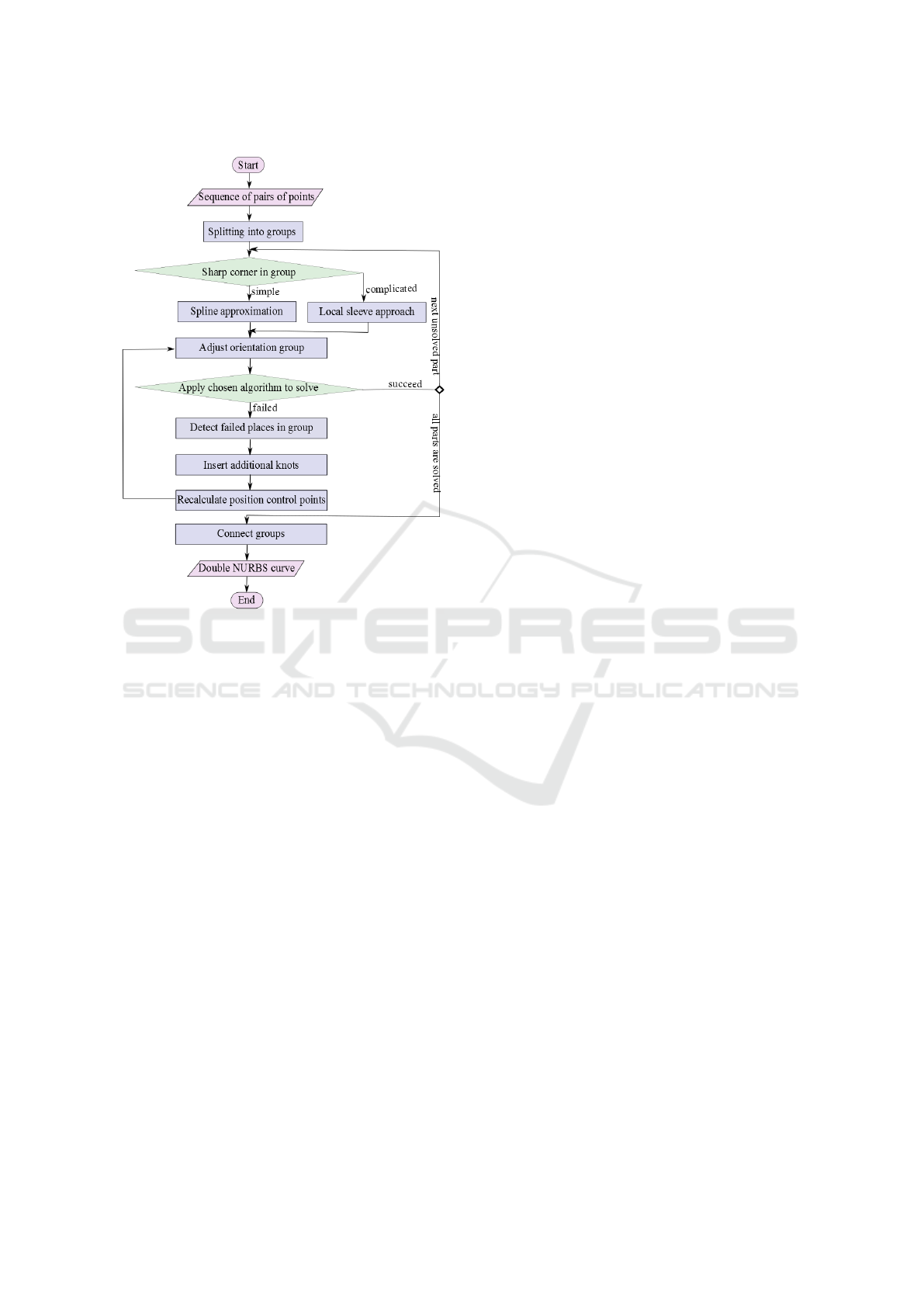
Figure 4: Outline of the process.
tion vectors (see Section 4.2). Based on the deci-
sion made for the position curve, use a modified
version of the respective algorithm that was ap-
plied to the position group to get the solution for
the orientation group (see Section 6).
4. If we obtain desired results we continue with the
next position group.
5. In case a solution could not be found, we need to
detect where the algorithm failed in the orienta-
tion group and decide where we need to insert ad-
ditional control points to form a constellation that
can be solved. Insert respective additional knots
in the knot vector and recalculate position control
points according to new knots (see Section 6).
6. For orientation group we regenerate orientation
vectors according to changed position control
points and resolve.
7. If all groups have been processed, connect all
groups to double NURBS curve (see Section 7).
4 ALLOCATING GROUPS
4.1 Splitting into Position Groups
As a first step, we need to partition the given se-
quence of position points into small curve segments.
The curve segments are represented as groups (or se-
quences) of consecutive input points. We want to
distinguish between simple and complicated groups.
As handling complicated groups will be done in a
more time-consuming processing step, it is desirable
to keep the number of complicated groups as small
as possible and to keep the complicated groups them-
selves as small as possible. A complex group is a
group that contains at least one sharp corner, i.e., an
angle smaller than a certain threshold α
sharp
. Conse-
quently, simple groups are those with no sharp cor-
ners. For complicated regions of the path we apply
the idea of threading splines through 3D channels (see
Section 5.1), for simple ones we use the idea of local
nonrational cubic approximation (see Section 5.2).
As processing time for groups increases superlin-
early with increasing group size, groups shall not ex-
ceed a certain upper limit of points n
max
. Also, very
long distances between consecutive points may make
it difficult to optimize for curvature. Hence, if two
consecutive input points exhibit a distance larger than
a certain threshold d
max
, the two points shall belong to
two different groups. If two successive groups have
not been separated by the maximum-distance crite-
rion, the two groups are close together and, in general,
have not been split in an area of low curvature. In this
case, it is likely that the optimization of the first group
generates a solution with the endpoint on the border
of the tolerance channel. This fact will make it hard
to produce a G
2
-continuous transition with low cur-
vature terms between the two groups. Thus, we want
the two groups to overlap, i.e., we want the groups to
share a small area. Consequently, we call this con-
nection an overlapping connection (see Fig. 5). De-
pending on which criterion caused the formation of a
group, we have different methods of how a group is to
be connected with the subsequent group when gener-
ating the overall curve. We distinguish between two
types of connections, namely a line connection and an
overlapping connection.
The algorithm of splitting points into groups was
described in (Selinger and Linsen, 2011).
4.2 Adjusting Orientation Groups
To solve the orientation part we first need to create
new initial orientation points based on the already op-
timized of position curve and given initial data. The
GRAPP 2018 - International Conference on Computer Graphics Theory and Applications
62
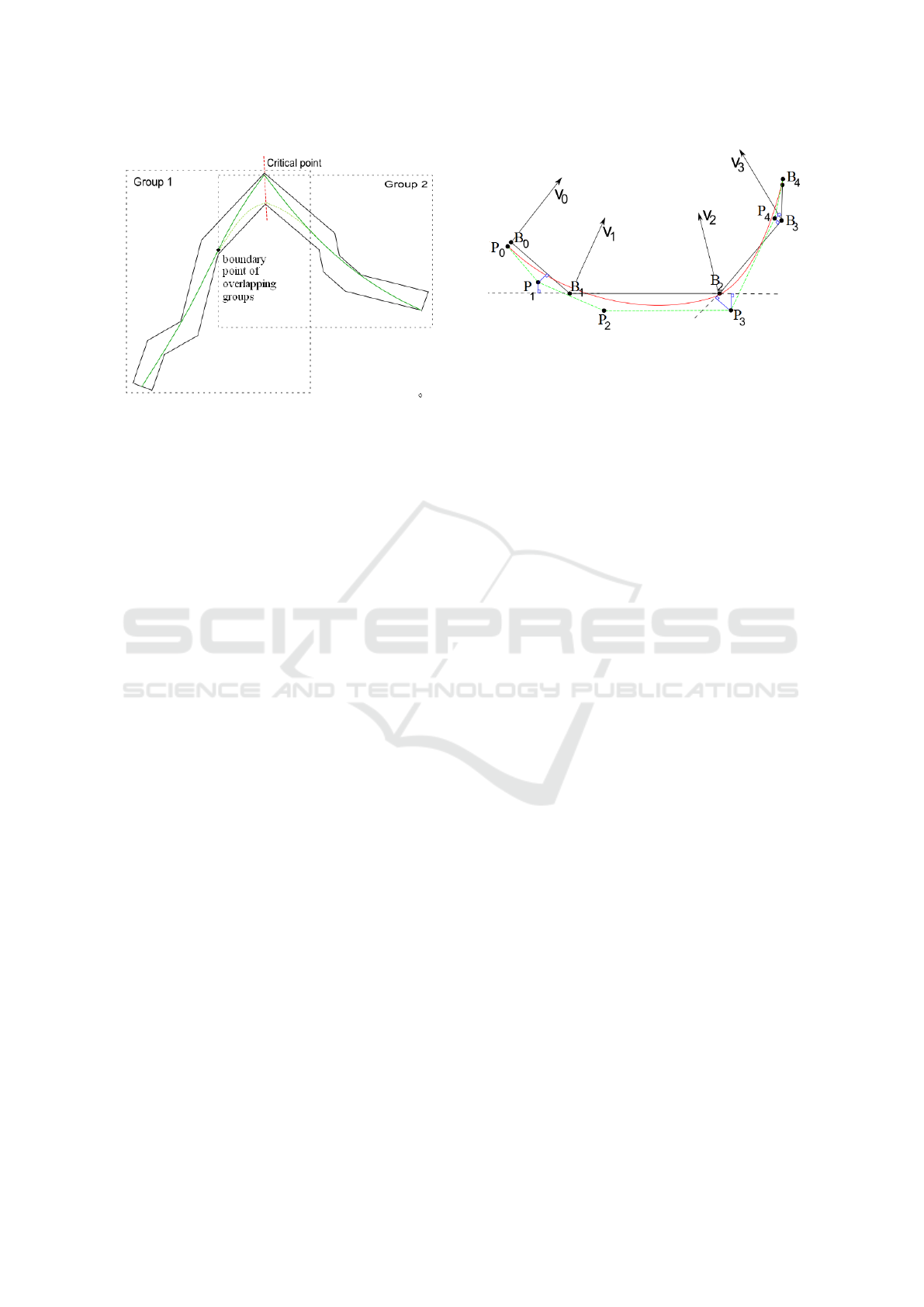
Figure 5: Necessity for overlapping connection at critical
area.
location of the new orientation points have to be cal-
culated in such a way that these points and the corre-
sponding position control points form new orientation
vectors. Direction of the vectors is considered as the
combination of the directions of the two closest ini-
tial vectors proportional to the distance between the
optimized position control point and the initial posi-
tion points which form these closest vectors. Given
a position control point, we detect to which interval
of initial position points the position control point be-
longs. We distinguish three different cases, which are
depicted in Fig. 6. For each control point P
i
we com-
pute lines that go through the control point P
i
and are
perpendicular to the lines of the initial position curve
B
0
,...,B
m
. We compute those perpendicular lines for
the closest two initial position curve segments B
i−1
B
i
and B
i
B
i+1
. We determine whether the intersection of
the perpendicular lines with the initial position curve
segments belong to the initial position curve. The fol-
lowing cases occur (cf. Fig. 6):
• Point P
1
: one of the perpendiculars at point P
1
in-
tersects with line B
0
B
1
inside interval (solid black
line) and another one intersects with outside part
of line B
1
B
2
(dashed black line). Hence, points P
1
lies in the first interval B
0
B
1
and the closest initial
orientation vector are V
1
,V
2
.
• Point P
3
: two perpendiculars at point P
3
intersect
with the lines B
1
B
2
and B
2
B
3
not inside the inter-
vals. Then, we compute the distances of the inter-
section point to the control point P
3
(blue lines)
and P
3
relates to that segment with shorter dis-
tance.
• Point P
4
: two perpendiculars at point P
4
inter-
sect with lines B
2
B
3
and B
3
B
4
inside the intervals.
Then, we again make the decision based on the
distance as in the preceding case.
Figure 6: Control points determination to a proper interval.
Arrows V
0
,...,V
4
indicate initial orientation vectors, where
the starting points of these vectors are the initial position
points B
0
,..., B
4
. P
0
,..., P
4
are optimized control points of
the local position B-spline curve (red curve), blue lines are
perpendiculars to lines formed by B
0
,..., B
4
.
After we have found the relating initial position
curve segment we built a new orientation vector from
the position control points with the direction linearly
interpolated between the closest initial vectors in pro-
portion to the distance from them to the current posi-
tion control point.
5 POSITION CURVE
OPTIMIZATION
In this section we present the algorithm for optimizing
the position curve. This is equivalent to the optimiza-
tion for 3-axis machining. Consequently, this step
is equivalent to the approach described previously
(Selinger and Linsen, 2011). For a comprehensive
description of the entire approach, we briefly describe
the main aspects of the algorithm. The main reason of
splitting data into groups is the superlinear time com-
plexity of the algorithm for complicated groups. We
have two types of connections between groups: lines
and overlapping. Separation of groups by line is ap-
plicable when the groups end at neighboring points
that are located in a distance more than some thresh-
old d
max
. Between these groups we can construct
a straight-line solution without spending any calcu-
lation time. Overlapping connections are necessary
when we have a large number of points close to each
other and collecting these points in one group might
increase running time of the algorithm significantly,
so we have to separate them. On the other hand, sep-
arating these points in different groups might occur in
areas with high curvature and it is not possible to have
feasible local solutions. In this case, we have overlap-
ping connections by including the same points at the
end of the first group and at the beginning of the sec-
ond group. Then, we can find solutions locally and
Efficient Curvature-optimized G
2
-continuous Path Generation with Guaranteed Error Bound for 5-axis Machining
63
the overlap assures a proper transition. For details we
refer to the literature (Selinger and Linsen, 2011).
5.1 Local Sleeve Approach for
Complicated Group
The handling of complicated groups is done by ex-
ecuting a local method based on the slefe approach
by Lutterkort and Peters (Myles and Peters, 2005;
Lutterkort and Peters, 1999a; Lutterkort and Peters,
1999b). Slefe is short for “subdividable linear effi-
cient function enclosure”. The idea is to generate two
polygons that represent lower and upper boundaries
of a given B-spline curve. The construction can be
generalized to curves in space by applying the con-
struction in both coordinate-axis directions of the un-
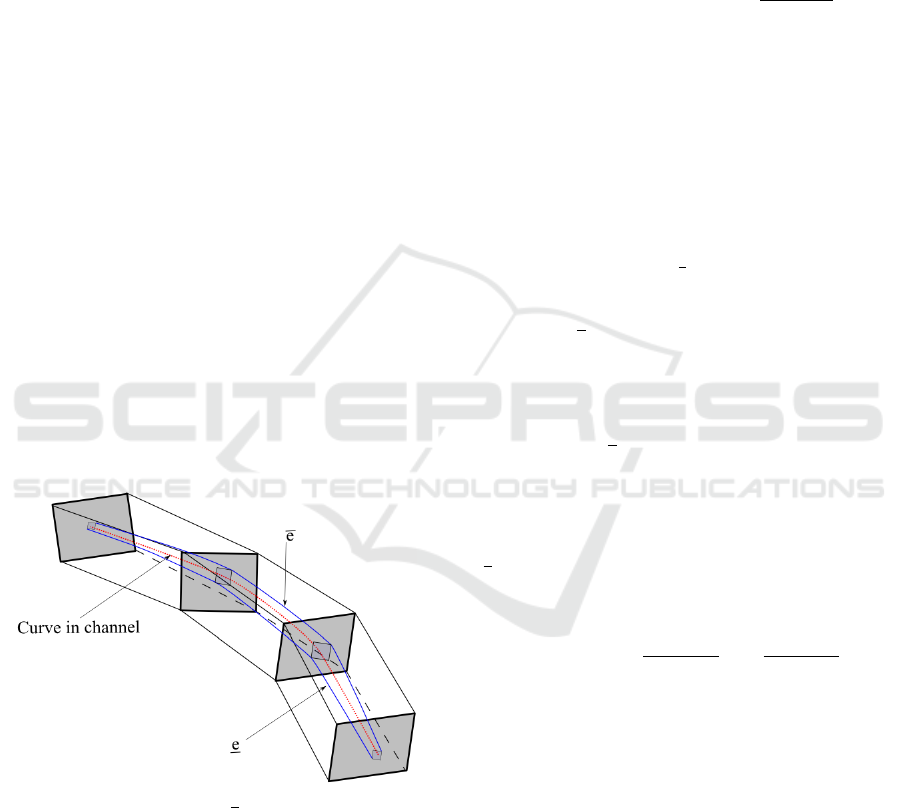
derlying 2D domain, see Fig. 7. It is, then, referred
to as the sleeve approach. After construction of the
piecewise linear sleeve, it is sufficient to constrain
this sleeve rather than the original nonlinear curve
to stay within the channel. Carefully formulated, this
approximation results in a linear feasibility problem
that is solvable using linear programming.
The construction of a sleeve around the spline
curve is equivalent to enclosing the spline curve with
linear pieces. However, in the channel problem, the
coefficients of the spline curve are unknown and are
sought as the solution of the feasibility problem.
Figure 7: Sleeve ¯e, e, and channel.
Given a B-spline curve
C(u) =
m
∑
j=0
P
j
N
d
j
(u),
with control points P
j
. Let the B-spline basis func-
tions N
d
j
of degree d be defined over a knot vector
(u
k
). The control polygon l(u) of the spline is the
piecewise linear interpolant to the control points P
j
at
the Greville abscissa
u
∗
j
=
j+d
∑
i= j+1
u
i
/d,
i.e. l(u
j
) = P
j
.
The weighted second differences ∆
2
P
i
of the con-
trol points are defined as
∆
2
P
i
= P
0
i+1
− P
0
i
, P
0
i
=
P
i
− P
i−1
u
∗
i
− u
∗
i−1
In addition, we define ∆
−
i
= min{0,∆
2
P
i
} and ∆
+
i
=
max{0,∆
2
P
i
}.
Over the interval [u
∗
k
,u
∗
k+1
] the contribution of the
i-th B-spline to the distance between a spline and its
control polygon is captured by the non-negative and
convex functions
β
ki
(u
∗
k
) :=
(
∑
¯
k
j=i
(u
∗
j
− u
∗
i
)N
d
j
, i > k,
∑
i
j=k
(u
∗
i
− u
∗
j
)N
d
j
, i ≤ k,
(3)
(4)
where
¯
k and k are the indices of the first and last ( at
most) d + 1 B-spline basis functions N
d
j
whose sup-
port spans u
∗
k
.
Then, we can formulate the restrictions for our
curve by
e(u) ≤ C(u) ≤ ¯e(u)
where
¯e(u) = l(u) + L (
∑
i
∆
+
i
β
ki
(u
∗
k
),
∑
i
∆
+
i
β
k+1,i
(u
∗
k+1
)),
e(u) = l(u) + L (
∑
i
∆
−
i
β
ki
(u
∗
k
),
∑
i
∆
−
i
β
k+1,i
(u
∗
k+1
)),
with u ∈ [u
∗
k
,u
∗
k+1
] and
L (a
1
,a
2
) = a
1
u
∗
k+1
− u
u
∗
k+1
− u
∗
k
+ a
2
u − u
∗
k
u
∗
k+1
− u
∗
k
.
The constraints force the sleeve, and thus the
spline, to stay inside the channel. We solve the
linear programming problem using a simplex ap-
proach. The target function we intend to minimize
is
∑
m−1
i=1
∑
j∈{x,y,z}
(∆
−
i, j
+ ∆
+
i, j
). By minimizing the ab-
solute second differences we are minimizing the cur-
vature of the spline. Sometimes the constraints cannot
be met. In this case, we need to insert further points
as described in Section 4.2.
5.2 Local G
2
- continuous Spline
Approximation for Simple Groups
Following the algorithm described in the approach
presented by Piegl (Piegl and Tiller, 1997) and its
GRAPP 2018 - International Conference on Computer Graphics Theory and Applications
64
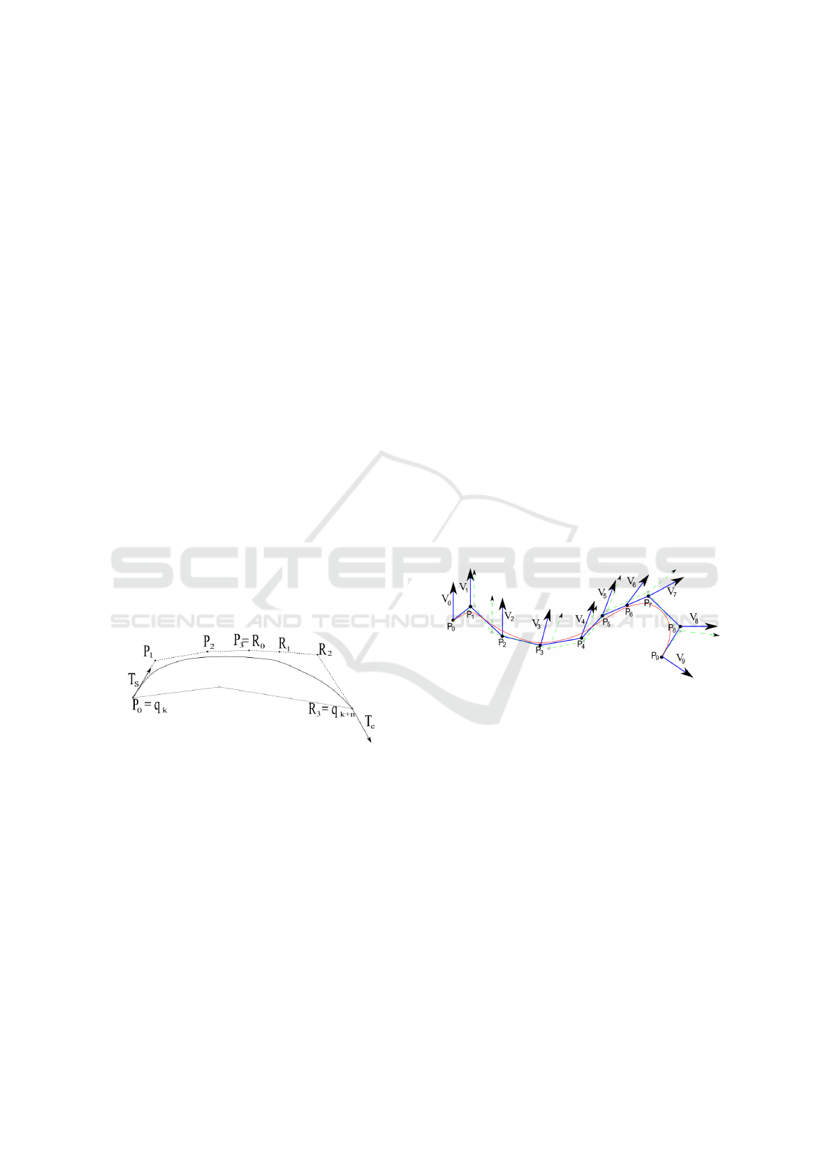
modifications presented in previous work (Selinger
and Linsen, 2011) we generate a local approxima-
tion scheme for simple groups using two cubic B
´
ezier
curves to assure G
2
-continuous connections. Given a
sequence of input points q
k
,..., q
k+n
, we set the first
control point of the first curve and the last control
point of the second curve to q
k
and q
k+n
, respectively.
Using the notations of Fig. 8, we set
P
0
= q
k
, R
3
= q
k+n
The endpoint interpolation property assures C
0
-
continuity. To assure G
1
-continuity, we set
P
1
= P
0
+ αT
s
and R
2
= R
3
+ βT
e
,
where T
s
and T
e
are the start and end unit tangents.
The unit tangents T
s
and T
e
as well as the values for
α and β are defined by the continuity constraints with
the preceding and succeeding group.
For G
2
-continuity at the group’s beginning we set
P
0
− 2P
1
+ P
2
= A,
where A is determined by the preceding group (or
A=0 for the first group, i.e., if k=0). The respective
continuity requirements where the two B
´
ezier curve
stitch together are given by
P
3
= R
0
,
P
2
− P
3
= R
0
− R
1
,
P
1
− 2P
2
+ P
3
= R
0
− 2R
1
+ R
2
.
Figure 8: Local nonrational cubic curve approximation.
To check for validity, we build the tolerance chan-
nel and the sleeve as described in Section 5.1. If the
sleeve lies inside the tolerance channel, the approxi-
mation is sufficiently precise. If not, we do the steps
described in Section 6 and then try to solve the prob-
lem for the modified sequence.
6 ORIENTATION CURVE
OPTIMIZATION
We want to generate a smooth B-spline curve for the
orientation of the milling tool based on the obtained
position curve and the newly generated orientation
vectors. We can see in Fig. 9 that the orientation
curve repeats the sharp angles of the position curve,
but we want to solve the orientation problem indepen-
dently from position curve. Therefore, we transform
the problem of finding the orientation control points
in space to the problem on the unit sphere. To re-
formulate the problem we start with orientation vec-
tors which are given as the difference between posi-
tion control points and respective interpolated orien-
tation points. We can imagine that the orientation op-
timization problem is defined on a sphere by moving
all position points to the sphere’s center (see Fig. 10).
After that we solve the problem with the same ap-
proach that was used for the position curve with the
modification that the tolerance channel is replaced by
a tolerance frustum, see Fig. 11. The frustum repre-
sents the tolerances for lead and tilt in the orientation
vector. They can be specified independently. In the
end we find the solution to the orientation curve by
adding the computed orientation vectors to the corre-
sponding position control points, i.e., by transforming
back from the sphere to the spatial representation. We
can do this operation without loss of continuity be-
cause by summing up corresponding control points of
the different B-spline curves we get a new B-spline
curve (see Fig. 12).
Figure 9: Green line connects initial position points, green
dashed vectors are initial orientation vectors, red line is a
B-spline position curve, blue line is control polygon of B-
spline position curve with control points P
0
,..., P
9
, blue vec-
tors V
0
,...,V
9
are generated new orientation vectors starting
from position control points.
To apply the local sleeve approach for compli-
cated groups and the spline approximation for simple
groups for solving the orientation curve problem we
have to modify a few parts. The main distinction from
the position curve optimization algorithm is using
the frustums to keep the control points inside them
(see Fig. 11). So, we need to add these constraints
additionally to the other restriction we have.
In some cases we might have an unfeasible orien-
tation group problem. To solve this problem we need
to achieve greater flexibility of the desired B-spline
curve by adding an additional control points. We find
a place in the orientation curve where the insertion of
Efficient Curvature-optimized G
2
-continuous Path Generation with Guaranteed Error Bound for 5-axis Machining
65
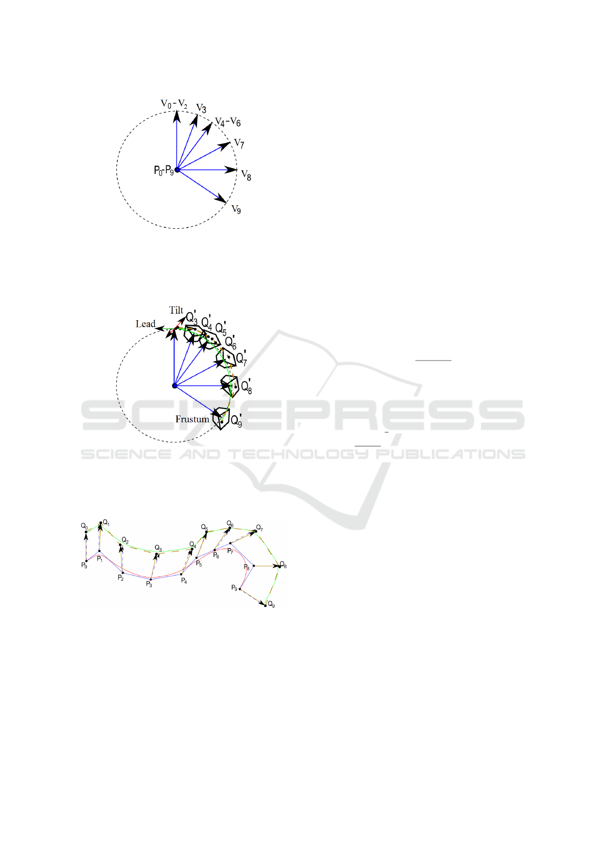
Figure 10: Described algorithms use the sphere representa-
tion to solve the orientation part of the problem. Generated
orientation vectors V
0
,...,V
9
from the Fig. 9 are placed at
the origin of a sphere such that, control points P
0
,..., P
9
co-
incide. We can see that V
0
,V
1
and V
2
are the same for this
example, because its have the same directions in Fig. 9.
Figure 11: Frustums are built around every vector to re-
strict control points Q
0
i
to lie inside these frustums. Con-
trol Points Q
0
4
,Q
0
5
,Q
0
6
lie inside matching frustums formed
around collinear vectors V
4
,V
5
,V
6
but they do not need to be
placed at the same position. Brown dashed line is a control
polygon Q
0
0
,..., Q
0
9
of green B-spline curve.
Figure 12: Obtained solution on the sphere is transformed
back to the initial problem using formula Q
i
= P
i
+ Q
0
i
.
Brown vectors are final orientation of the tool, red line is a
position B-spline curve, green line is a orientation B-spline
curve, dashed brown line is a control polygon of orientation
curve. The two B-spline curves have the same knot vector.
a new additional control point is required. Usually
the solution fails in places where we have a longer
distance between some control points than in the rest
of the group. Thus, we want to insert new control
points in the middle of this distance. Then, we in-
sert a respective knot in the existing knot vector and
recalculate dependent control points for the position
sequence of the control points, build new orientation
vectors for the changed points, and resolve the orien-
tation group. Thus, even if we have to insert addi-
tional control points in the orientation curve, we keep
proper orientation vectors.
The procedure of the point insertion for position
B-spline curve C(u) as in Equation (1) with a knot
vector U as in Equation (2) is the following (Piegl
and Tiller, 1997):
Given a knot ¯u ∈ [u
k
,u
k+1
) that we want to insert into
U to form the new knot vector U
0
= (u
0
0
= u
0
,...,u
0
k
=
u
0
k
,u
0
k+1
= ¯u,u
0
k+2
= u
0
k+1
,...,u
0
m+1
= u
m
), we recal-
culate the control points using Equation (5) by
P
0
k−d
= P
k−d
,
P
0
i
= αP
i
+ (1 − α)P
i−1
, k − d + 1 ≤ i ≤ k,
P
0
k+1
= P
k
.
For i = k − d + 1,...,k we have
α =
¯u − u
i
u
i+d
− u
i
(5)
We need to generate a new control point in the middle
of the interval P
i−1
P
i
then build a new orientation vec-
tor from this point and frustum around it to get an ori-
entation control point at the desired place. To achieve
this, we set α =
1
2
. Hence, from Equation (5) we ob-
tain u =
u
i+d
+u
i
2
. Afterwards, we recalculate points
P
0
i−d+1
,...,P
0
i
and try to solve the orientation problem
again.
7 COMBINING GROUPS
To complete the process we need to put all groups to-
gether in two B-spline curves with common knot vec-
tor. We have to assure G
2
-continuity at the connec-
tions. To fulfill G
2
-continuity requirements in case
of a line connection, we insert three additional points
lying on the line a
k
a
k+1
, where neighboring initial
points a
k
and a
k+1
belong to different groups. We ad-
just two groups by adding the three additional points
to the end of the first group (i.e., after a
k
) and to the
beginning of the second group (i.e., before a
k+1
).
For an overlapping connection of two groups, we
need to distinguish whether the first group is a com-
plicated or a simple one. If the first group is a com-
plicated group, we calculate a new control point ly-
ing on the curve. We obtain this by double knot in-
sertion (see (Selinger and Linsen, 2011)), cutting off
the control points after this point, and adjusting the
knot sequence by removing knots after the inserted
GRAPP 2018 - International Conference on Computer Graphics Theory and Applications
66
ones. The second group will then start with the last
control point of the first group. We did not mod-
ify the shape of the first group’s curve. If the first
group is a simple group, we delete the last few control
points until we find a control point that was an input
point. Since B
´
ezier curves are endpoint interpolating,
we can start the second group with that control point.
When solving for the second group, we have to pick
the first three control points of that group such that
G
2
-continuity is achieved. G
0
-continuity requires that
the last control point of the first group has to be equal
to the first control point of the second group, for G
1
-
continuity we need to have the proportional tangent
vector of the adjacent parts, and the G
2
-continuity
condition requires equality of the second derivatives
of the adjacent parts. Using notations of Fig. 13, we
obtain:
P
k
= R
1
,
P
k−1
− P
k
||P
k−1
,P
k
||
=
R
1
− R
2
||R
1
,R
2
||
,
P
k−2
− 2P
k−1
+ P
k
= R
1
− 2R
2
+ R
3
.
Figure 13: Connecting groups with G
2
-continuity.
The procedure of combining groups is described
in (Selinger and Linsen, 2011) in details for position
curves in 3-axis matching and it is the same for orien-
tation curve.
8 RESULTS AND DISCUSSION
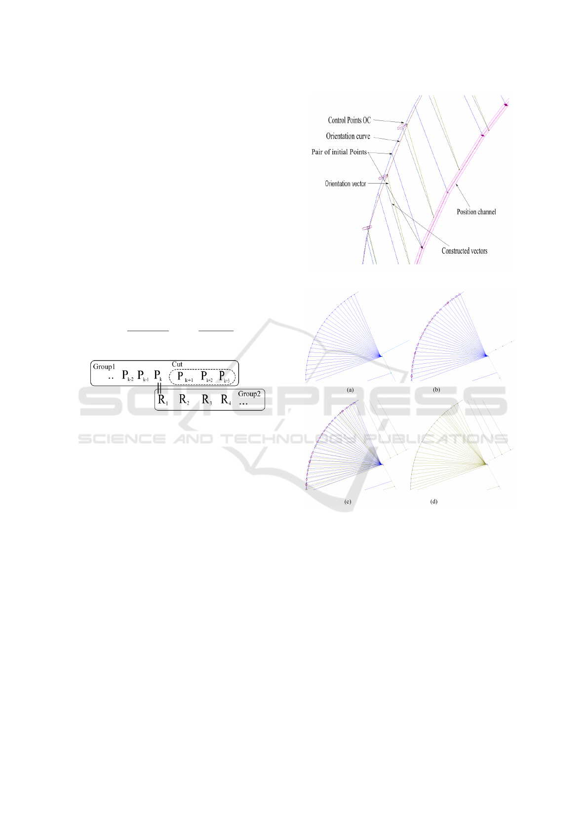
In Fig. 14 we show a zoomed-in version of a real 5-
axis tool path that was optimized with our approach.
We can observe the correctness of the solution. Gen-
erated orientation vectors have similar directions as
the initial ones and control points of the orientation
curve stay inside the frustums.
Fig. 15 depicts the individual steps of the op-
timization of the 5-axis tool path for a 90
◦
turn.
Using initial data of orientation curve and control
points of the position curve, we build frustums around
the newly generated orientation vectors from position
control points and get a solution with orientation con-
trol points inside the corresponding frustum.
Next, we want to investigate the computation time
of our approach. For our experiments, we used a
workpiece which mostly consists of almost straight
Figure 14: Optimized 5-axis tool path.
Figure 15: Outline of the process of generating a 5-axis tool
path optimization for a 90
◦
turn. (a) Initial position and ori-
entation data. (b) Constructed frustums. (c) Generated ori-
entation vectors and curve. (d) Resulting B-spline curves.
parts, rounded parts, and turns as shown in Fig. 16
with 209 input pairs of position and orientation points.
Computation time for the 5-axis orientation algorithm
is 0.735 seconds with the tolerance of the channel be-
ing 0.0008 mm and lead and tilt tolerance being 0.1
◦
.
The respective 3-axis optimization when only consid-
ering the position curve takes 0.38 seconds with the
same tolerance of the channel. It takes less than dou-
ble time to compute double amount of initial points
because for almost straight areas of orientation parts
on the sphere we have a very simple solution which
we can get right away or we need to insert much less
(or even none) additional points when compared to
the position part.
Efficient Curvature-optimized G
2
-continuous Path Generation with Guaranteed Error Bound for 5-axis Machining
67
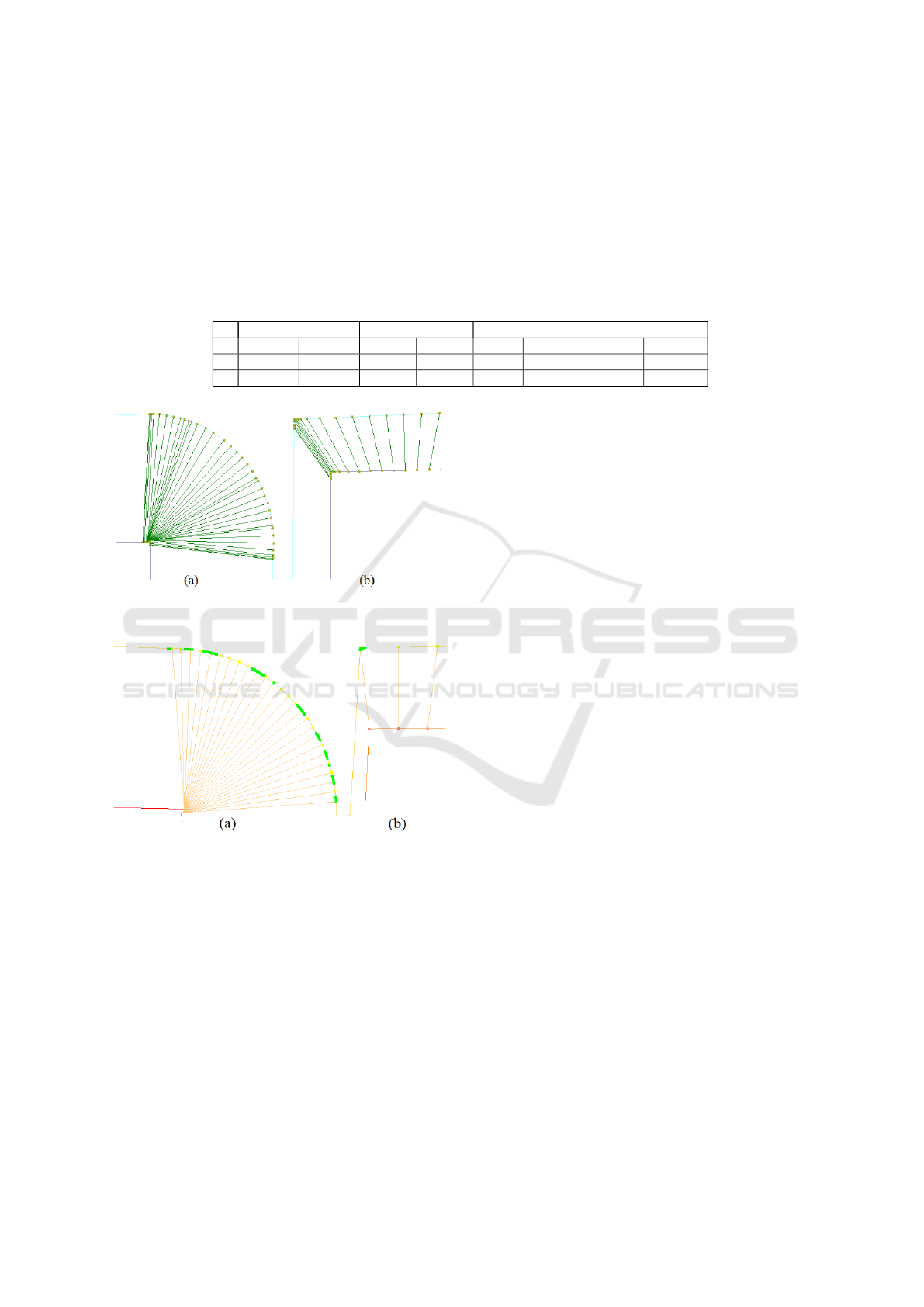
Table 1: Maximum and average curvature of parts of the workpiece parts separated in groups by type of initial data: line,
simple parts with almost straight lines, rounded parts, and turns with small angles (see Fig. 16). In the first test (upper row)
we use tolerances of lead and tilt equal to 0.5
◦
, in the second test (lower row) the tolerances are 1.2
◦
.
We calculate the average and maximum curvature (Selinger and Linsen, 2011) of the orientation B-spline curve separately for
different parts of the workpiece. Table 1 lists the computed curvature values. The upper row was calculated using tolerances
of lead and tilt equal to 0.5
◦
, the lower row using tolerances equal to 1.2
◦
. We can observe that for line and simple parts the
tolerances of lead and tilt do not influence the curvature because the solution is simple and control points are lying inside a
smaller frustum anyway. However, for rounded parts and turns we have high values of curvature and the higher values are
obtained for smaller angle tolerances, because the curve is forced to make sharper turns. These tests were performed on the
workpiece shown in Fig. 17.
line parts simple parts rounded parts parts with turn
av max av max av max av max
1 1.8e-10 9.4e-10 0.0018 0.0377 1.111 2.2009 18.615 329.435
2 1.8e-10 9.4e-10 0.0018 0.0377 1.105 2.0455 18.3175 311.257
Figure 16: Parts of the workpiece. (a) Rounded parts (b)
Turns and almost straight parts.
Figure 17: Parts of the workpiece. High curvature (higher
than one) of the orientation curve are highlighted by green
points, red line is a position B-spline curve, orange lines are
orientation vectors and orientation polygon. (a) Rounded
parts. (b) Turns.
We also calculate the deviation of the resulting
orientation vectors from the interpolated orientation
vectors in terms of lead and tilt. We denote by vec-
tor D the forward direction of the lead, where D is in
the forward direction of the curve, −D is the back-
ward direction of the lead. The vector R denotes the
right direction of the tilt, where R is computed by the
cross-product D × O, where O is the orientation vec-
tor of the curve. Left direction of the tilt is the di-
rection −R. For the lead, we compute the ratio of
the angle between the resulting orientation vector and
the plane that is formed by the left and right points
of the frustum, and the given angle of lead tolerance.
This ratio is 0 if the interpolated orientation vector
and the resulting orientation vector are equal, and 1 if
the maximum tolerance is used. The sign of the ratio
indicates whether the orientation has been changed in
forward or backward direction. Respectively for tilt,
we compute the ratio of the angle between the result-
ing orientation vector and the plane that is formed by
forward and backward points of the frustum, and the
given angle of tilt tolerance
We can observe that for part of the workpiece as
in Fig. 18 with allowed lead and tilt tolerance of 1
◦
the values of deviation are not very high (see Fig. 19).
However, if we decrease the allowed tolerance to 0.1
◦
we can see that deviation for some parts of the work-
piece can reach to 100% in one direction and after
that very quickly to the other direction (see Fig. 21).
This effect can be explained by the example shown
in Fig. 20. In Fig. 20, we show the orientation vectors
from Fig. 18 on the sphere. The first few cyan orienta-
tion vectors and its frustums are almost identical. The
subsequent vectors of different red colors are start-
ing to slightly change the direction inside the same
frustums. The reason is to keep the orientation curve
straight. The resulting orientation vectors are located
in one plane, but the positions are slightly changing in
the direction of the subsequent frustum.
On the workpiece with rounded parts and turns the
deviation of the resulting vectors are shown in Fig. 22.
For the rounded part in Fig. 22a, we can see zoomed-
in picture in Fig. 23a, and for Fig. 22b the view from
the top is in Fig. 23b. In Fig. 23a, we can see that the
orientation vectors are frequently changing its posi-
tions with respect to the generated vectors due to the
minimization of the sum of the second differences. In
Fig. 23b, one can observe that the resulting deviation
vectors before the turn changed the side with respect
to the polygon formed by the centers of the frustums
in order to to decrease the curvature.
GRAPP 2018 - International Conference on Computer Graphics Theory and Applications
68
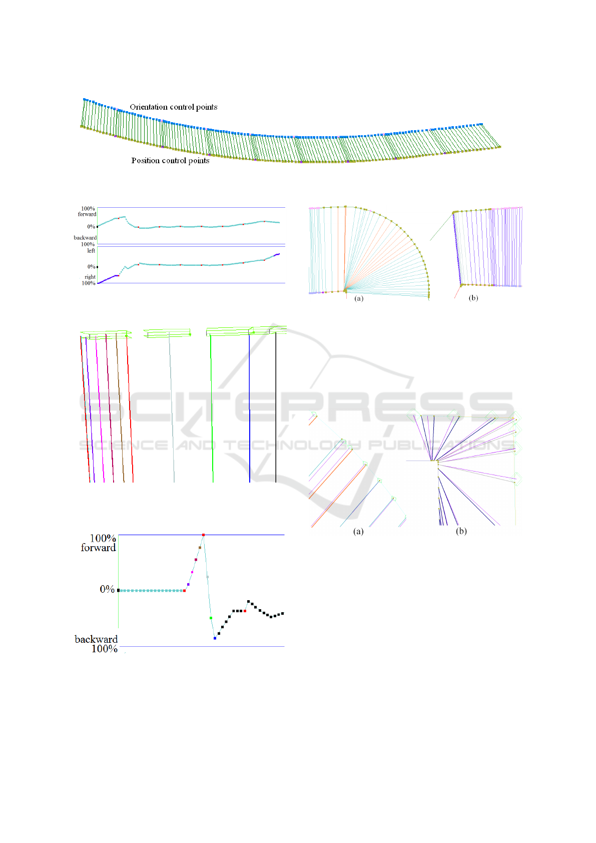
Figure 18: Part of the workpiece. Yellow points are control points of the position curve, blue are orientation control points.
Pink points are connection points between groups. Green lines are orientation vectors.
Figure 19: Diagram of lead (upper) and tilt (lower) devia-
tion of the orientation vectors for a given tolerance of 1
◦
for
both lead and tilt and the example in Fig. 18.
Figure 20: Resulting vectors and its frustums for problem
transformed into the sphere problem. All orientation vec-
tors (lines of different color) start from one position, which
is the center of the sphere.
Figure 21: Diagram of lead deviation of the resulting vec-
tors on the sphere for the example in Fig. 18. Color of the
points is the same as the color of the corresponding vector
in Fig. 20. Given tolerance is 0.1
◦
for lead and tilt.
Figure 22: Parts of the workpiece. Points are control points,
red curve is position B-spline curve, green curve is orienta-
tion B-spline curve. (a) Straight and rounded parts. Cyan
and orange vectors are unit resulting orientation vectors,
which indicate delay or overdrive of the resulting orienta-
tion vector in comparison to the to initial one. (b) Turns.
Dark purple and gray vectors are unit resulting orientation
vectors. Different colors indicate different sides of the poly-
gon formed by centers of the frustums.
Figure 23: Parts of the workpiece. Purple lines are inter-
polated orientation vectors. (a) Zoomed-in rounded part,
see Fig. 22a. Orange lines are resulting vectors with delay,
light blue are resulting vectors with overdrive. (b) View of
the turn from the top, see Fig. 22b. Gray and dark purple
lines are resulting vectors on opposite sides of the polygon.
As parameters for our experiments, we define dis-
tance measures as multiples of the tolerance of the
channel ε, which is half of the width of the chan-
nel. A good tradeoff in terms of computation time for
solving individual groups and for splitting and joining
overhead was found by setting the maximum number
n
max
of points per group to n
max
= 50. A good value
for the distance threshold d
max
for splitting into sep-
arate groups was found to be d
max
= 300ε. An angle
is reported as a sharp corner, iff its cosine is smaller
Efficient Curvature-optimized G
2
-continuous Path Generation with Guaranteed Error Bound for 5-axis Machining
69

than cos(α
sharp
) = −0.85, because for corners that are
sharper than this value the oscillation increases signif-
icantly when we apply the local spline approximation
method.
9 CONCLUSIONS
We developed an algorithm for generating curvature-
optimized tool paths for 5-axis milling. The gener-
ated tool paths consist of a position B-spline curve
and an orientation B-spline curve. The position curve
can be handles like a 3-axis machining tool path. For
the orientation curve, the control points are restricted
to stay within a frustum formed by the lead and tilt
tolerances. To obtain an acceptable quality-speed ra-
tio, we combine two algorithms: a local version of
the sleeve-algorithm and a local spline approximation
with G
2
-continuity connections. Corresponding po-
sition and orientation point groups are solved by the
same algorithm. We solve the orientation problem on
the sphere to avoid any complications caused by loca-
tion of position points. The splitting of the original
orientation curve into groups is performed with re-
spect to the corresponding position point groups and
complexity of the groups. The local spline approxi-
mation algorithm is very efficient and produces good
results for simple groups, while the local sleeve algo-
rithm is less efficient but produces high-quality results
even for complicated groups.
The created algorithm can be used as a part of a
micro milling process. This approach provides new
possibilities for calculating velocity, acceleration, and
jerk profiles. The benefits are that profiles are easier
to compute and that the milling can generally be per-
formed with a higher velocity. The latter is essential
for practical purposes, since the higher the velocity of
the tool tip is the faster is the manufacturing process.
ACKNOWLEDGMENTS
This work was supported by BMWi under grant num-
ber 5166/50258.
REFERENCES
Robert V. Fleisig and Allan D. Spence (2001) Constant feed
and reduced angular acceleration interpolation algo-
rithm for multi-axis machining. Computer Aided De-
sign 33(1):1-15.
Cha-Soo Jun, Kyungduck Cha, Yuan-Shin Lee (2003) Op-
timizing tool orientations for 5-axis machining by
configuration-space search method. Computer-Aided
Design 35(6):549-566.
Taejung Kim and Sanjay E. Sarma (2002) Toolpath gen-
eration along directions of maximum kinematic per-
formance; a first cut at machine-optimal paths.
Computer-Aided Design 34(6): 453-468.
Jean Marie Langeron, Emmanuel Duc, Claire Lartigue,
Pierre Bourdet (2004) A new format for 5-axis tool
path computation, using B-spline curves. Computer-
Aided Design 36(12): 1219-1229.
Sylvain Lavernhe, Christophe Tournier and Claire Lartigue
(2007) Kinematical performance prediction in multi-
axis machining for process planning optimization.
The International Journal of Advanced Manufacturing
Technology 37(5-6): 534-544.
Wei Li, Yadong Liu, Kazuo Yamazaki, Makoto Fujisima
and Masahiko Mori (2008) The design of a NURBS
pre-interpolator for five-axis machining. The Interna-
tional Journal of Advanced Manufacturing Technol-
ogy 36(9-10):927-935.
Xianbing Liua, Fahad Ahmada, Kazuo Yamazakia, and
Masahiko Mori (2005) Adaptive interpolation scheme
for NURBS curves with the integration of machining
dynamics. International Journal of Machine Tools and
Manufacture 45(4-5):433-444.
David Lutterkort and J
¨
org Peters (1999) Tight lin-
ear envelopes for splines. Numerische Mathematik
89(4):735-748.
David Lutterkort and J
¨
org Peters (1999) Smooth path in
a polygon channel. In: Proceedings of the 15th an-
nual symposium on Computational Geometry 316-
321, ACM Press.
Ashish Myles and J
¨
org Peters (2005) Threading splines
through 3D channels. Computer-Aided Design
37(2):139-148.
J
¨
org Peters and Xiaobin Wu (2004) Sleeves for planar spline
curves. Computer-Aided Design 21(6):615-635.
Les A. Piegl (1991) On NURBS: a Survey. IEEE Computer
Graphics and Applications 11(1):55-71.
Les A. Piegl and Wayne Tiller (1997) The NURBS Book.
Springer.
Les A. Piegl and Wayne Tiller (2002) Data approximation
using biarcs. 18:59-65. Engineering with Computers,
Springer.
Hartmut Prautzsch, Wolfgang Boehm and Marco Paluszny
(2002) B
´
ezier and B-Spline Techniques. Springer.
Selinger, Jevgenija and Linsen, Lars (2011) Efficient
Curvature-optimized G2-continuous Path Generation
with Guaranteed Error Bound for 3-axis Machining.
in Proceedings of the 15th International Conference
on Information Visualisation 519–527. 5th Interna-
tional Conference on Geometric Modeling and Imag-
ing (GMAI 2011) . IEEE Computer Society.
Rong Zhen Xu, Le Xie, Cong Xin Li, and Dao Shan Du
(2008) Adaptive parametric interpolation scheme with
limited acceleration and jerk values for NC machin-
ing. The International Journal of Advanced Manufac-
turing Technology 36(3-4):343-354.
Wang Yongzhang, Ma Xiongbo, Chen Liangji, Han Zhenyu
(2007) Realization Methodology of a 5-axis Spline In-
terpolator in an Open CNC System. Chinese Journal
of Aeronautics 20(4):362-369.
GRAPP 2018 - International Conference on Computer Graphics Theory and Applications
70
